Smoothed Histograms
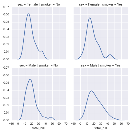
I recently picked up Seaborn for data visualization. It’s very user friendly.
One of my favorite plots is the Kernel Density Estimation (KDE) plot. And this post is about how KDE is generated.
Probability Density Estimation
There are 2 general approaches to estimating the PDF of a distribution.
The first group is parametric. We have some prior assumption that the data follows a certain distribution (e.g. gaussian, student t, gamma) and try to fit parameters around these distributions.
The second is nonparametric. They make no prior assumptions on the distribution of the data by modeling the data instead of the parameters. I will go into more details the Parzen Window approach.
(Edited December 15, 2016 - There are also the mixture model that combines parametric and nonparametric approaches, e.g. fitting Mixture of Gaussians with EM)
The General Approach
The PDF of x can be modeled as the following:
Here v stands for the volume. First, we specify a bin size (or volume), like we do with histograms.
Then we get k (the number of samples in the bin) and n (the total number of samples) to calculate the density of the bin.
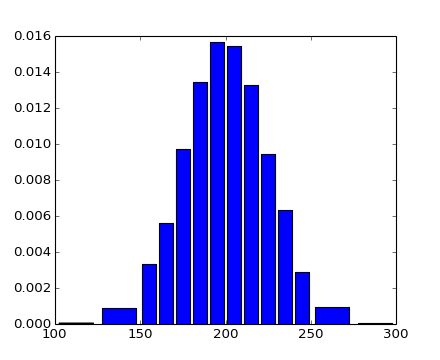
Overall, the formula works exact like a histogram, but converted (via division over the volume / bin size) to make it behave like density.
Parzen Window
The Parzen Window is a very simplistic kernel that is best explained pictorially.

Source
Here the 7 points are colored. The density estimation is:
Here the denom is $ 21 = nv = 7 * 3 $
This way of calculating density is nonparametric because we need to remember every single sample in $ D $.
Smoothed Parzen Window
Instead of a kernel that returns 0 or 1, we can use a gaussian instead
As a result, the generated density estimation is smoothed.

Choosing the Right Window Size
The window size h is the only parameter that we need to decide for the KDE.

Generally, if h is too big (left) or h is too small (right), then the quality of the density estimation will suffer.
In a classification context, we can systematically choose h by fitting KDEs to each category, classify test points under the maximum posterier, and varying h to get the best accuracy.
Conclusion
Check out the kdeplot function in Seaborn. Hopefully this post explained the basics of how the density estimation really works.