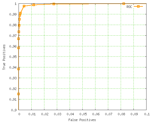
ROC Curve
Most of us use the ROC curve to assess our binary classifiers everyday. Sometimes we take for granted its theoretical properties. In this post, I will take some time and analyze why the properties are what they are.

2 properties will be covered:
-
The baseline is the diagonal line
-
The area can be interpreted as how strong the classifier is
1. The baseline is the diagonal line
So as we know, the x-axis of the ROC curve is the False Positive Rate (FPR) and the y-axis is the True Positive Rate (TPR).
If we have a dataset with $\pi \in [0,1] $ positives, and $ 1 - \pi $ in the negatives, and we predict randomly with a positive rate of $ p $ and negative rate of $ 1 - p $, then we can calculate the TPR and FPR as a ratio.
Since TPR and FPR are both p, a random classifier (baseline) will have a ROC curve of slope 1 (the diagonal) and an AUC of 0.5.
2. The area can be interpreted as how strong the classifier is
Technically, the area is a bit different from I described.
Let’s go into why.
The integral means that for each negative example, count the number of positive examples with a higher score than this negative example.
If we have a perfect classifier, then all P positives will be scored higher than the negative example, so the integral will result in a maximum area of $ P * N$.

Note: Intuitively, the perfect classifier has {TPR = 1 and FPR = 0}, which is the upper left point
Combined together, the 2 terms give us a nice interpretation of the $A_{AUC} \in [0,1] $ as the classifier’s ability to discern positive and negative data.
Conclusion
Unfortunately, I did not go over other properties such as linear correlation with accuracy, pareto optimality and relationships with the calibration curve. That’s for another day.
The 2 main properties outlined in this post make the ROC curve a fairly good way to compare binary classifiers. These are great theoretical advantages that other popular metrics (such as the precision-recall or the calibration curves) don’t have.