The fast and easy guide to the most popular Deep Learning framework in the world.
TensorFlow is a framework created by Google for creating Deep Learning models. Deep Learning is a category of machine learning models that use multi-layer neural networks. The idea of deep learning has been around since 1943 when neurophysiologist Warren McCulloch and mathematician Walter Pitts wrote a paper on how neurons might work and they model a simple neural network using electrical circuits.
Many, many developments have occurred since then. These highly accurate mathematical models are extremely computationally expensive. With recent advances in processing power from GPUs and increasing CPU power Deep Learning has been exploding with popularity.
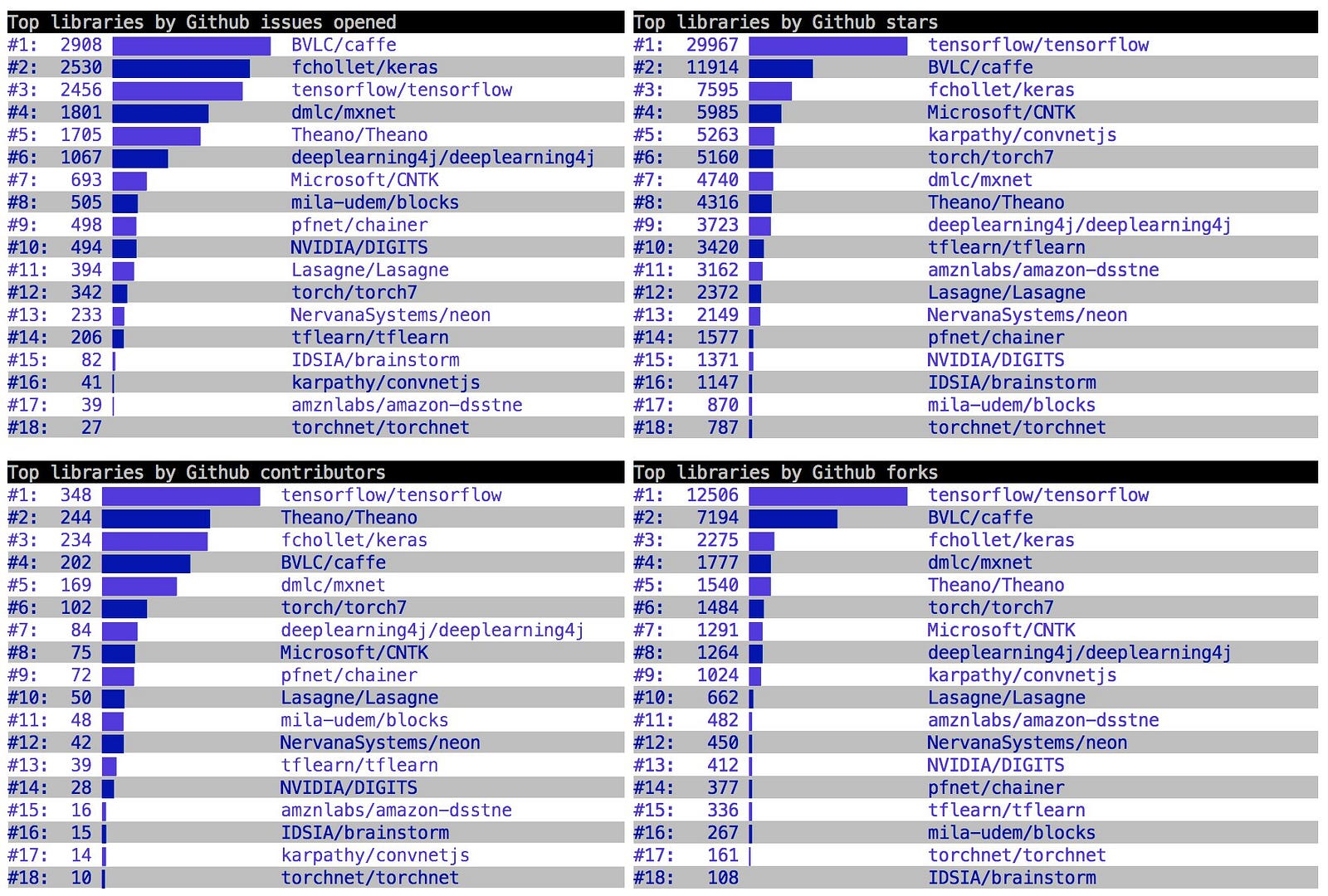
TensorFlow was created with processing power limitations in mind. Open sourced in November 2015, this library can be ran on computers of all kinds including smartphones. It allows for instant creation of trained production models. It is currently the number 1 Deep Learning framework at the time of writing this article.

Basic Computational Graph
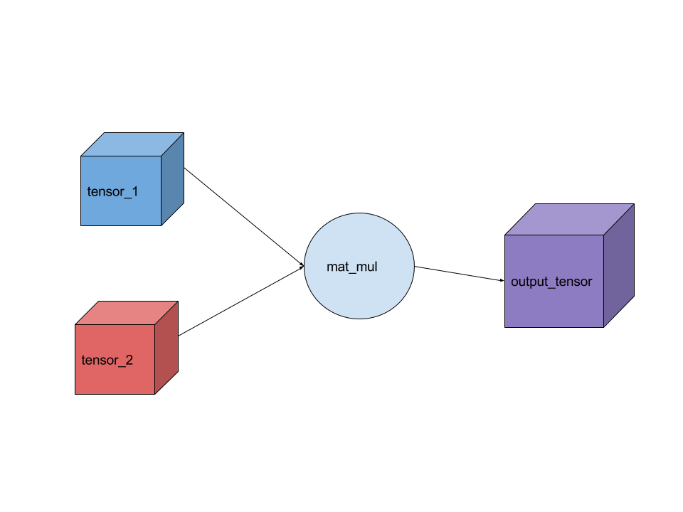
Everything in TensorFlow is based on creating a computational graph. If you’ve ever used Theano then this section will look familiar. Think of a computational graph as a network of nodes, with each node known as an operation, running some function that can be as simple as addition or subtraction to as complex as some multi variate equation.
An Operation also referred to as op can return zero or more tensors which can be used later on in the graph. Heres a list of operations with their output for example
Each operation can be handed a constant, array, matrix or n-dimensional matrix. Another word for an n-dimensional matrix is a tensor, a 2-dimensional tensor is equivalent to a m x m matrix.

Our computational graph The code above is creating two constant tensors and multiplying them together and outputting our result. This is a trivial example that demonstrates how you can create a graph and run the session. All inputs needed by the op are run automatically. They’re typically ran in parallel. This session run actually causes the execution of three operations in the graph, creating the two constants then the matrix multiplication.
Graph
The constants and operation that we created above was automagically added to the graph in TensorFlow. The graph default is intantiated when the library is imported. Creating a Graph object instead of using the default graph is useful when creating multiple models in one file that do not depend on each other.
any variables or operations used outside of the with new_graph.as_default() will be added to the default graph that is created when the library is loaded. You can even get a handle to the default graph with
for most cases it’s best to stick with the default graph.
Session
There are two kinds of Session objects in TensorFlow:
tf.Session()
This encapsulates teh environment that operations and tensors are executed and evaluated. Sessions can have their own variables, queues and readers that are allocated. So it’s important to use the close() method when the session is over. There are 3 arguments for a Session, all of which are optional.
-
target — The execution engine to connect to.
-
graph — The Graph to be launched.
-
config — A ConfigProto protocl buffer with configuration options for the session
To have run one “step” of the TensorFlow computation this function is called and all of the necessary dependencies for the graph to execute are ran.
tf.InteractiveSession()
This is the exact same as tf.Session() but is targeted for using IPython and Jupyter Notebooks that allows you to add things and use Tensor.eval() and Operation.run() instead of having to do Session.run() every time you want something to be computed.
InteractiveSession allows so that you dont have to explicitly pass Session object.
Variables
Variables in TensorFlow are managed by the Session. They persist between sessions which are useful because Tensor and Operation objects are immutable. Variables can be created by tf.Variable().
most of the time you will want to create these variables as tensors of zeros, ones or random values:
-
tf.zeros() — creates a matrix full of zeros
-
tf.ones() — creates a matrix full of ones
-
tf.random_normal() — a matrix with random uniform values between an interval
-
tf.random_uniform() — random normally distributed numbers
-
tf.truncated_normal() — same as random normal but doesn’t include any numbers more than 2 standard deviations.
These functions take an inital shape parameter where the dimension of the matrix is defined. For example:
To have your variable set to one of these matrix helper functions:
To have these variables initialized you must use TensorFlow’s variable initialization function then pass it to the session. This way when multiple sessions are ran the variables are the same.
If you’d like to completely change the value of a variable you can use Variable.assign() operation, this must be run in a session update the value.
Sometimes you would like to add a counter inside your model this is where you can do a Variable.assign_add() method which takes a numeric parameter and increments it by the parameter. Similarily there is Variable.assign_sub().
Scope
To control the complexity of models and make them easier to break down into individual pieces TensorFlow has scopes. Scopes are very simple and even help break down your model when using TensorBoard (which will be covered in Part 2). Scopes can even be nested inside of other scopes.
Scopes may not seem that powerful right now but used in collaboration with TensorBoard and they’re very useful.
Conclusion
I’ve demonstrated many of the building blocks that TensorFlow offers. These individual pieces added together can create very complicated models. There is much more that TensorFlow offers, if there are any requests for features in upcoming parts let me know.
Also published on Medium.
