Decision Trees Tutorial

Would you survive a disaster?

Certain groups of people, such as women and children, might be entitled to receiving help first, granting them a higher chance of survival. Knowing whether you belong to one of these privileged groups would help predict whether you would make it out alive. To identify which groups have higher survival rates, we can use decision trees.

While we forecast the rate of survival here, decision trees are used in a a wide range of applications. In the business setting, it can be used to define customer profiles or to predict who would resign.

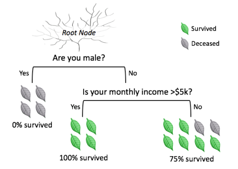
A decision tree leads you to a prediction by asking a series of questions on whether you belong to certain groups (see Figure 1). Each question must only have 2 possible responses, such as “yes” versus “no”. You start at the top question, called the root node, then move through the tree branches according to which groups you belong to, until you reach a leaf node. The proportion of survivors at that leaf node would be your predicted chance of survival.

Figure 1. Example decision tree.

Decision trees are versatile, as they can handle questions about categorical groupings (e.g. male vs. female) or about continuous values (e.g. income). If the question is about a continuous value, it can be split into groups – for instance, comparing values which are “above average” versus “below average”.

In standard decision trees, there should only be two possible responses, such as “yes” versus “no”. If we want to test three or more responses (“yes”, “no”, “sometimes”), we can simply add more branches down the tree (see Figure 2).

Figure 2. Testing multiple categories in a decision tree.

We use passenger data for the ill-fated cruise liner, the Titanic, to check if certain groups of passengers were more likely to have survived. The dataset was originally compiled by the British Board of Trade to investigate the ship’s sinking. The data used in this example is a subset of the original, and is one of the in-built datasets freely available in R.

Computing a decision tree to predict survival rates generates the following:

Figure 3. Predict whether you’d survive the sinking of Titanic.

From the result, it seems that you would have a good chance of being rescued from the Titanic if you were a female from 1st/2nd class cabin, or a male child from 1st/2nd class cabin.

Decision trees are popular because they are easy to interpret. The question is, how is a decision tree generated?

A decision tree is grown by first splitting all data points into two groups, with similar data points grouped together, and then repeating the binary splitting process within each group. As a result, each subsequent leaf node will have fewer but more homogeneous data points. The basis of decision trees is that by isolating groups of “survivors” via different paths in the tree, anyone else belonging to those paths would be predicted to be a likely “survivor” as well.

The process of repeatedly partitioning the data to obtain homogeneous groups is called recursive partitioning. It involves just 2 steps, illustrated in the animated GIF below:

Step 1: Identify the binary question that splits data points into two groups that are most homogeneous.

Step 2: Repeat Step 1 for each leaf node, until a stopping criterion is reached.

There are various possible stopping criteria:

– Stop when data points at the leaf are all of the same predicted category/value– Stop when the leaf contains less than five data points– Stop when further branching does not improve homogeneity beyond a minimum threshold

Stopping criteria are selected using cross-validation to ensure that the decision tree can draw accurate predictions for new data.* (If you’re unfamiliar with cross-validation, stay tuned – it will be explained in a future post. To be notified of new posts, sign up at the end of this tutorial.)*

As recursive partitioning only uses the best binary questions to grow a decision tree, the presence of non-significant variables would not affect results. Moreover, binary questions impose a central divide to split data points, so decision trees are robust against extreme values (i.e. outliers).

Using the best binary question to split the data at the start may not lead to the most accurate predictions. Sometimes, less effective splits used initially may lead to even better predictions subsequently.

To resolve this, we can choose different combinations of binary questions to grow multiple trees, and then use the aggregated prediction of those trees. This technique is called a random forest. Or, instead of combining binary questions randomly, we can strategically select them, such that the prediction accuracy for each subsequent tree improves incrementally. Then, a weighted average of predictions from all trees is taken. This technique is called gradient boosting.

While random forest and gradient boosting tend to produce more accurate predictions, their complexity renders the solution harder to visualize. Hence, they are often called “black-boxes”. On the other hand, predictions from a decision tree can be examined using a tree diagram. Learning which predictors are important allows us to plan more targeted interventions.

Did you learn something useful today? We would be glad to inform you when we have new tutorials, so that your learning continues!

Like this:

Like Loading…

Related