This is the first in a series of posts about recurrent neural networks in Tensorflow. In this post, we will build a vanilla recurrent neural network (RNN) from the ground up in Tensorflow, and then translate the model into Tensorflow’s RNN API.

Edit 2017/03/07: Updated to work with Tensorflow 1.0.

Introduction to RNNs

RNNs are neural networks that accept their own outputs as inputs. So as to not reinvent the wheel, here are a few blog posts to introduce you to RNNs:

Written Memories: Understanding, Deriving and Extending the LSTM, on this blog
Recurrent Neural Networks Tutorial, by Denny Britz
The Unreasonable Effectiveness of Recurrent Neural Networks, by Andrej Karpathy
Understanding LSTM Networks, by Christopher Olah

Outline of the data

In this post, we’ll be building a no frills RNN that accepts a binary sequence X and uses it to predict a binary sequence Y. The sequences are constructed as follows:

Input sequence (X): At time step t, (X_t) has a 50% chance of being 1 (and a 50% chance of being 0). E.g., X might be [1, 0, 0, 1, 1, 1 … ].
Output sequence (Y): At time step t, (Y_t) has a base 50% chance of being 1 (and a 50% base chance to be 0). The chance of (Y_t) being 1 is increased by 50% (i.e., to 100%) if (X_{t-3}) is 1, and decreased by 25% (i.e., to 25%) if (X_{t-8}) is 1. If both (X_{t-3}) and (X_{t-8}) are 1, the chance of (Y_{t}) being 1 is 50% + 50% - 25% = 75%.

Thus, there are two dependencies in the data: one at t-3 (3 steps back) and one at t-8 (8 steps back).

This data is simple enough that we can calculate the expected cross-entropy loss for a trained RNN depending on whether or not it learns the dependencies:

If the network learns no dependencies, it will correctly assign a probability of 62.5% to 1, for an expected cross-entropy loss of about 0.66.
If the network learns only the first dependency (3 steps back) but not the second dependency, it will correctly assign a probability of 87.5%, 50% of the time, and correctly assign a probability of 62.5% the other 50% of the time, for an expected cross entropy loss of about 0.52.
If the network learns both dependencies, it will be 100% accurate 25% of the time, correctly assign a probability of 50%, 25% of the time, and correctly assign a probability of 75%, 50% of the time, for an expected cross extropy loss of about 0.45.

Here are the calculations:

import numpy as np

print("Expected cross entropy loss if the model:")
print("- learns neither dependency:", -(0.625 * np.log(0.625) +
 0.375 * np.log(0.375)))
# Learns first dependency only ==> 0.51916669970720941
print("- learns first dependency: ",
 -0.5 * (0.875 * np.log(0.875) + 0.125 * np.log(0.125))
 -0.5 * (0.625 * np.log(0.625) + 0.375 * np.log(0.375)))
print("- learns both dependencies: ", -0.50 * (0.75 * np.log(0.75) + 0.25 * np.log(0.25))
 - 0.25 * (2 * 0.50 * np.log (0.50)) - 0.25 * (0))

Expected cross entropy loss if the model:

learns neither dependency: 0.661563238158
learns first dependency: 0.519166699707
learns both dependencies: 0.454454367449 ```

Model architecture

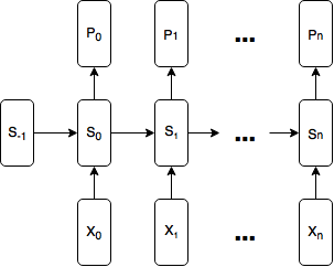
The model will be as simple as possible: at time step t, for (t \in {0, 1, \dots n}) the model accepts a (one-hot) binary (X_t) vector and a previous state vector, (S_{t-1}), as inputs and produces a state vector, (S_t), and a predicted probability distribution vector, (P_t), for the (one-hot) binary vector (Y_t).

Formally, the model is:

(S_t = \text{tanh}(W(X_t \ @ \ S_{t-1}) + b_s))

(P_t = \text{softmax}(US_t + b_p))

where (@) represents vector concatenation, (X_t \in R^2) is a one-hot binary vector, (W \in R^{d \times (2 + d)}, \ b_s \in R^d, \ U \in R^{2 \times d}), (b_p \in R^2) and d is the size of the state vector (I use (d = 4) below). At time step 0, (S_{-1}) (the initial state) is initialized as a vector of zeros.

Here is a diagram of the model:

How wide should our Tensorflow graph be?

To build models in Tensorflow generally, you first represent the model as a graph, and then execute the graph. A critical question we must answer when deciding how to represent our model is: how wide should our graph be? How many time steps of input should our graph accept at once?

Each time step is a duplicate, so it might make sense to have our graph, G, represent a single time step: (G(X_t, S_{t-1}) \mapsto (P_t, S_t)). We can then execute our graph for each time step, feeding in the state returned from the previous execution into the current execution. This would work for a model that was already trained, but there’s a problem with using this approach for training: the gradients computed during backpropagation are graph-bound. We would only be able to backpropagate errors to the current timestep; we could not backpropagate the error to time step t-1. This means our network will not be able to learn how to store long-term dependencies (such as the two in our data) in its state.

Alternatively, we might make our graph as wide as our data sequence. This often works, except that in this case, we have an arbitrarily long input sequence, so we have to stop somewhere. Let’s say we make our graph accept sequences of length 10,000. This solves the problem of graph-bound gradients, and the errors from time step 9999 are propagated all the way back to time step 0. Unfortunately, such backpropagation is not only (often prohibitively) expensive, but also ineffective, due to the vanishing / exploding gradient problem: it turns out that backpropagating errors over too many time steps often causes them to vanish (become insignificantly small) or explode (become overwhelmingly large). To understand why this is the case, we apply the chain rule repeatedly to (\frac{\partial E_t}{\partial S_{t-k}}) and observe that there is a product of (k) factors (Jacobian matrices) linking the gradient at (S_t) and the gradient as (S_{t-k}):

[\frac{\partial E_t}{\partial S_{t-k}} =

\frac{\partial S_t}{\partial S_{t-k}} =

\frac{\partial E_t}{\partial S_t}

\left(\frac{\partial S_t}{\partial S_{t-1}}

\frac{\partial S_{t-1}}{\partial S_{t-2}} \dots

\frac{\partial S_{t-k+1}}{\partial S_{t-k}}\right) =

\frac{\partial E_t}{\partial S_t}

\prod_{i=1}^{k}\frac{\partial S_{t-i+1}}{\partial S_{t-i}}]

In the words of Pascanu et al., “in the same way a product of [k] real numbers can shrink to zero or explode to infinity, so does this product of matrices …” See On the difficulty of training RNNs, by Pascanu et al. or my post Written Memories: Understanding, Deriving and Extending the LSTM for more detailed explanations and references.

The usual pattern for dealing with very long sequences is therefore to “truncate” our backpropagation by backpropagating errors a maximum of (n) steps. We choose (n) as a hyperparameter to our model, keeping in mind the trade-off: higher (n) lets us capture longer term dependencies, but is more expensive computationally and memory-wise.

A natural interpretation of backpropagating errors a maximum of (n) steps means that we backpropagate every possible error (n) steps. That is, if we have a sequence of length 49, and choose (n = 7), we would backpropagate 42 of the errors the full 7 steps. This is not the approach we take in Tensorflow. Tensorflow’s approach is to limit the graph to being (n) units wide. See Tensorflow’s writeup on Truncated Backpropagation (“[Truncated backpropagation] is easy to implement by feeding inputs of length [(n)] at a time and doing backward pass after each iteration.”). This means that we would take our sequence of length 49, break it up into 7 sub-sequences of length 7 that we feed into the graph in 7 separate computations, and that only the errors from the 7th input in each graph are backpropagated the full 7 steps. Therefore, even if you think there are no dependencies longer than 7 steps in your data, it may still be worthwhile to use (n > 7) so as to increase the proportion of errors that are backpropagated by 7 steps. For an empirical investigation of the difference between backpropagating every error (n) steps and Tensorflow-style backpropagation, see my post on Styles of Truncated Backpropagation.

Using lists of tensors to represent the width

Our graph will be (n) units (time steps) wide where each unit is a perfect duplicate, sharing the same variables. The easiest way to build a graph containing these duplicate units is to build each duplicate part in parallel. This is a key point, so I’m bolding it: the easiest way to represent each type of duplicate tensor (the rnn inputs, the rnn outputs (hidden state), the predictions, and the loss) is as a list of tensors. Here is a diagram with references to the variables used in the code below:

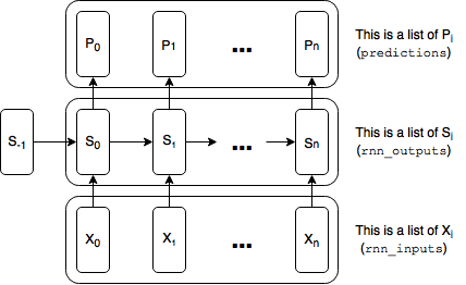
We will run a training step after each execution of the graph, simultaneously grabbing the final state produced by that execution to pass on to the next execution.

Without further ado, here is the code:

Imports, config variables, and data generators

import numpy as np
import tensorflow as tf
%matplotlib inline
import matplotlib.pyplot as plt

Global config variables

num_steps = 5 # number of truncated backprop steps (‘n’ in the discussion above) batch_size = 200 num_classes = 2 state_size = 4 learning_rate = 0.1

def gen_data(size=1000000):
 X = np.array(np.random.choice(2, size=(size,)))
 Y = []
 for i in range(size):
 threshold = 0.5
 if X[i-3] == 1:
 threshold += 0.5
 if X[i-8] == 1:
 threshold -= 0.25
 if np.random.rand() > threshold:
 Y.append(0)
 else:
 Y.append(1)
 return X, np.array(Y)

# adapted from https://github.com/tensorflow/tensorflow/blob/master/tensorflow/models/rnn/ptb/reader.py
def gen_batch(raw_data, batch_size, num_steps):
 raw_x, raw_y = raw_data
 data_length = len(raw_x)

 # partition raw data into batches and stack them vertically in a data matrix
 batch_partition_length = data_length // batch_size
 data_x = np.zeros([batch_size, batch_partition_length], dtype=np.int32)
 data_y = np.zeros([batch_size, batch_partition_length], dtype=np.int32)
 for i in range(batch_size):
 data_x[i] = raw_x[batch_partition_length * i:batch_partition_length * (i + 1)]
 data_y[i] = raw_y[batch_partition_length * i:batch_partition_length * (i + 1)]
 # further divide batch partitions into num_steps for truncated backprop
 epoch_size = batch_partition_length // num_steps

 for i in range(epoch_size):
 x = data_x[:, i * num_steps:(i + 1) * num_steps]
 y = data_y[:, i * num_steps:(i + 1) * num_steps]
 yield (x, y)

def gen_epochs(n, num_steps):
 for i in range(n):
 yield gen_batch(gen_data(), batch_size, num_steps)

Model

Placeholders
"""

x = tf.placeholder(tf.int32, [batch_size, num_steps], name='input_placeholder')
y = tf.placeholder(tf.int32, [batch_size, num_steps], name='labels_placeholder')
init_state = tf.zeros([batch_size, state_size])

RNN Inputs
"""

# Turn our x placeholder into a list of one-hot tensors:
# rnn_inputs is a list of num_steps tensors with shape [batch_size, num_classes]
x_one_hot = tf.one_hot(x, num_classes)
rnn_inputs = tf.unstack(x_one_hot, axis=1)

””” Definition of rnn_cell

This is very similar to the call method on Tensorflow’s BasicRNNCell. See: https://github.com/tensorflow/tensorflow/blob/master/tensorflow/contrib/rnn/python/ops/core_rnn_cell_impl.py#L95 “”” with tf.variable_scope(‘rnn_cell’): W = tf.get_variable(‘W’, [num_classes + state_size, state_size]) b = tf.get_variable(‘b’, [state_size], initializer=tf.constant_initializer(0.0))

def rnn_cell(rnn_input, state): with tf.variable_scope(‘rnn_cell’, reuse=True): W = tf.get_variable(‘W’, [num_classes + state_size, state_size]) b = tf.get_variable(‘b’, [state_size], initializer=tf.constant_initializer(0.0)) return tf.tanh(tf.matmul(tf.concat([rnn_input, state], 1), W) + b)

"""
Adding rnn_cells to graph

This is a simplified version of the "static_rnn" function from Tensorflow's api. See:
https://github.com/tensorflow/tensorflow/blob/master/tensorflow/contrib/rnn/python/ops/core_rnn.py#L41
Note: In practice, using "dynamic_rnn" is a better choice that the "static_rnn":
https://github.com/tensorflow/tensorflow/blob/master/tensorflow/python/ops/rnn.py#L390
"""
state = init_state
rnn_outputs = []
for rnn_input in rnn_inputs:
 state = rnn_cell(rnn_input, state)
 rnn_outputs.append(state)
final_state = rnn_outputs[-1]

””” Predictions, loss, training step

Losses is similar to the “sequence_loss” function from Tensorflow’s API, except that here we are using a list of 2D tensors, instead of a 3D tensor. See: https://github.com/tensorflow/tensorflow/blob/master/tensorflow/contrib/seq2seq/python/ops/loss.py#L30 “””

#logits and predictions with tf.variable_scope(‘softmax’): W = tf.get_variable(‘W’, [state_size, num_classes]) b = tf.get_variable(‘b’, [num_classes], initializer=tf.constant_initializer(0.0)) logits = [tf.matmul(rnn_output, W) + b for rnn_output in rnn_outputs] predictions = [tf.nn.softmax(logit) for logit in logits]

Turn our y placeholder into a list of labels

y_as_list = tf.unstack(y, num=num_steps, axis=1)

#losses and train_step losses = [tf.nn.sparse_softmax_cross_entropy_with_logits(labels=label, logits=logit) for \ logit, label in zip(logits, y_as_list)] total_loss = tf.reduce_mean(losses) train_step = tf.train.AdagradOptimizer(learning_rate).minimize(total_loss)

Train the network
"""

def train_network(num_epochs, num_steps, state_size=4, verbose=True):
 with tf.Session() as sess:
 sess.run(tf.global_variables_initializer())
 training_losses = []
 for idx, epoch in enumerate(gen_epochs(num_epochs, num_steps)):
 training_loss = 0
 training_state = np.zeros((batch_size, state_size))
 if verbose:
 print("\nEPOCH", idx)
 for step, (X, Y) in enumerate(epoch):
 tr_losses, training_loss_, training_state, _ = \
 sess.run([losses,
 total_loss,
 final_state,
 train_step],
 feed_dict={x:X, y:Y, init_state:training_state})
 training_loss += training_loss_
 if step % 100 == 0 and step > 0:
 if verbose:
 print("Average loss at step", step,
 "for last 250 steps:", training_loss/100)
 training_losses.append(training_loss/100)
 training_loss = 0

 return training_losses

training_losses = train_network(1,num_steps) plt.plot(training_losses)

EPOCH 0
Average loss at step 100 for last 250 steps: 0.6559883219
Average loss at step 200 for last 250 steps: 0.617185292244
Average loss at step 300 for last 250 steps: 0.595771013498
Average loss at step 400 for last 250 steps: 0.568864737153
Average loss at step 500 for last 250 steps: 0.524139249921
Average loss at step 600 for last 250 steps: 0.522666031122
Average loss at step 700 for last 250 steps: 0.522012578249
Average loss at step 800 for last 250 steps: 0.519179680347
Average loss at step 900 for last 250 steps: 0.519965928495

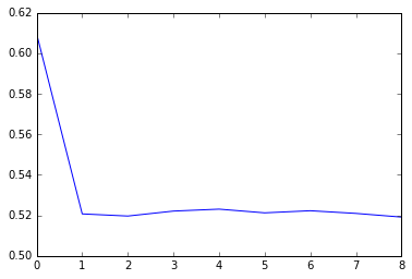
As you can see, the network very quickly learns to capture the first dependency (but not the second), and converges to the expected cross-entropy loss of 0.52.

Exporting our model to a separate file in order to play with hyperparameters, we can see what happens when we use num_steps = 1 and num_steps = 10 (for this latter case, we also increase the state_size so as to maintain the the information about the second dependency for the required 8 steps):

import basic_rnn
def plot_learning_curve(num_steps, state_size=4, epochs=1):
 global losses, total_loss, final_state, train_step, x, y, init_state
 tf.reset_default_graph()
 g = tf.get_default_graph()
 losses, total_loss, final_state, train_step, x, y, init_state = \
 basic_rnn.setup_graph(g,
 basic_rnn.RNN_config(num_steps=num_steps, state_size=state_size))
 res = train_network(epochs, num_steps, state_size=state_size, verbose=False)
 plt.plot(res)

NUM_STEPS = 1 “”” plot_learning_curve(num_steps=1, state_size=4, epochs=2)

![](https://r2rt.com/static/images/RNN_output_25_0.png)

NUM_STEPS = 10 “”” plot_learning_curve(num_steps=10, state_size=16, epochs=10)

![](https://r2rt.com/static/images/RNN_output_26_0.png)

As expected, using `num_steps = 10` comes close to our expected cross-entropy for knowing both dependencies (0.454). However, using `num_steps = 1` hovers around something slightly better than the expected cross-entropy for knowing neither dependency (0.66), and doesn’t seem to converge. What’s going on?

The answer is that some information about the first dependency is making its way into the incoming state by pure chance. Although the model can’t learn weights that will maintain information about the first dependency (due to the backpropagation being graph-bound), it can learn to take advantage of whatever information about \(X_{t-3}\) is left over in \(S_{t-1}\). In doing so, the model changes the way information about \(X_{t-3}\) is stored in \(S_{t-1}\), which explains why the loss goes up and down, rather than settling at a local minima.

### Translating our model to Tensorflow

Translating our model to Tensorflow’s API is easy. We simply replace these two sections:

””” Definition of rnn_cell

””” Adding rnn_cells to graph

This is a simplified version of the “static_rnn” function from Tensorflow’s api. See: https://github.com/tensorflow/tensorflow/blob/master/tensorflow/contrib/rnn/python/ops/core_rnn.py#L41 Note: In practice, using “dynamic_rnn” is a better choice that the “static_rnn”: https://github.com/tensorflow/tensorflow/blob/master/tensorflow/python/ops/rnn.py#L390 “”” state = init_state rnn_outputs = [] for rnn_input in rnn_inputs: state = rnn_cell(rnn_input, state) rnn_outputs.append(state) final_state = rnn_outputs[-1]

With these two lines:

cell = tf.contrib.rnn.BasicRNNCell(state_size) rnn_outputs, final_state = tf.contrib.rnn.static_rnn(cell, rnn_inputs, initial_state=init_state)

### Using a dynamic RNN

Above, we added every node for every timestep to the graph before execution. This is called “static” construction. We could also let Tensorflow dynamically create the graph at execution time, which can be more efficient. To do this, instead of using a list of tensors (of length `num_steps` and shape `[batch_size, features]`), we keep everything in a single 3-dimnesional tensor of shape `[batch_size, num_steps, features]`, and use Tensorflow’s `dynamic_rnn` function. This is shown below.

### Final model — static

To recap, here’s the entire static model, as modified to use Tensorflow’s API:

Placeholders “””

x = tf.placeholder(tf.int32, [batch_size, num_steps], name=’input_placeholder’) y = tf.placeholder(tf.int32, [batch_size, num_steps], name=’labels_placeholder’) init_state = tf.zeros([batch_size, state_size])

Inputs “””

x_one_hot = tf.one_hot(x, num_classes) rnn_inputs = tf.unstack(x_one_hot, axis=1)

RNN “””

cell = tf.contrib.rnn.BasicRNNCell(state_size) rnn_outputs, final_state = tf.contrib.rnn.static_rnn(cell, rnn_inputs, initial_state=init_state)

Predictions, loss, training step “””

with tf.variable_scope(‘softmax’): W = tf.get_variable(‘W’, [state_size, num_classes]) b = tf.get_variable(‘b’, [num_classes], initializer=tf.constant_initializer(0.0)) logits = [tf.matmul(rnn_output, W) + b for rnn_output in rnn_outputs] predictions = [tf.nn.softmax(logit) for logit in logits]

y_as_list = tf.unstack(y, num=num_steps, axis=1)

losses = [tf.nn.sparse_softmax_cross_entropy_with_logits(labels=label, logits=logit) for \ logit, label in zip(logits, y_as_list)] total_loss = tf.reduce_mean(losses) train_step = tf.train.AdagradOptimizer(learning_rate).minimize(total_loss)

### Final model — dynamic

And here it is with the `dynamic_rnn` API, which should be preferred over the static API:

Placeholders “””

Inputs “””

rnn_inputs = tf.one_hot(x, num_classes)

RNN “””

cell = tf.contrib.rnn.BasicRNNCell(state_size) rnn_outputs, final_state = tf.nn.dynamic_rnn(cell, rnn_inputs, initial_state=init_state)

Predictions, loss, training step “””

with tf.variable_scope(‘softmax’): W = tf.get_variable(‘W’, [state_size, num_classes]) b = tf.get_variable(‘b’, [num_classes], initializer=tf.constant_initializer(0.0)) logits = tf.reshape( tf.matmul(tf.reshape(rnn_outputs, [-1, state_size]), W) + b, [batch_size, num_steps, num_classes]) predictions = tf.nn.softmax(logits)

losses = tf.nn.sparse_softmax_cross_entropy_with_logits(labels=y, logits=logits) total_loss = tf.reduce_mean(losses) train_step = tf.train.AdagradOptimizer(learning_rate).minimize(total_loss) ```

Conclusion

And there you have it, a basic RNN In Tensorflow. In the next post of this series, we’ll look at how to improve our base implementation, how to upgrade to a GRU/LSTM or other custom RNN cell and use multiple layers, how to add features like dropout and layer normalization, and how to use our RNN to generate sequences.

Recurrent Neural Networks in Tensorflow I

Silviu Pitis