So far, our policy has simply been to act greedily on some value function. What if we tried to learn the policy itself? We can represent this policy as the probability to take a certain action, given the state.
π = P (a s)
This brings with it some advantages and disadvantages. In the case of very high-dimension action spaces, it can take a lot of computing power to find the maximum value, and learning a policy allows us to bypass that step. We also get the benefit of stochasticity, or a random probability to choose one action compared to another. In some partially observed environments, random decision making is an essential piece of the optimal strategy. However, learning a policy often has higher variance and will take longer to train, and it may reach a local optima.

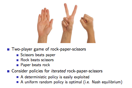
example of stochastic (random) policy being superior
So, how do we learn a policy? We’ll assume some function π[W] (s,a) that takes in state-action pairs and returns probabilities. W represents parameters that we use to learn this function. If we’re using a neural network, W is the weights of the network.
I won’t go into too much of the mathematical details here, so check out the relevant video in David Silver’s RL course for derivations and stuff.
In short, if we know the gradient of parameters to make the probability of taking action A from state S more likely, we adjust the parameters in that direction to the scale of the return for taking the action.
Let’s go over a short example using Monte-Carlo learning. To learn a policy, we would first have to wait until the end of the episode. For every timestep, we would update parameter W:
1 | |
Note that total reward means from that timestep onwards.
This is great and all, but we run into same problems as using Monte-Carlo learning in the past: since we wait until the end of the episode, variance is high. To solve this, we can use good old policy evaluation to estimate the value function, and bootstrap off of that. This is known as actor-critic, where the actor is the policy and the critic is a value function.
An simple actor-critic follows the steps below:
-
Estimate value function V(s) using policy evaluation of π
-
Take an action based on policy π
-
Find TD error of that action:
-
update parameters W to the scale of TD error
1 | |
To understand how this works, think of reward + discountFactor * V(next state) as the value of taking action A from state S, or Q(s,a).
The TD error can then be thought of as Q(s,a) - V(s), or “how good is it to take this action from this state, relative to how good the state is?”.
Let’s say we’re in a state with a value of 100, we take an action that rewards us with 10, and the next state has a discounted value of 95. (95 + 10) - 100 = 5, so this was clearly a good move. Therefore, we should update the policy in a direction that would increase the probability to take that action from that state.
This works really well since a bigger TD error would have a greater impact on our policy, and negative TD errors would adjust parameters in the opposite direction, decreasing the probability of taking a bad action.
Note: this is a continuation from a previous post, with information taken from David Silver’s RL Course.