TensorFlow Implementation of "A Neural Algorithm of Artistic Style"

This notebook and code are available on Github.

This notebook illustrates a Tensorflow implementation of the paper “A Neural Algorithm of Artistic Style” which is used to transfer the art style of one picture to another picture’s contents.

If you like to run this notebook, you will need to install TensorFlow, Scipy and Numpy. You will need to download the VGG-19 model. Feel free to play with the constants a bit to get a feel how the bits and pieces play together to affect the final image generated.

1
2
3
4
5
6
7
8
9
10
11
12
# Import what we need
import os
import sys
import numpy as np
import scipy.io
import scipy.misc
import tensorflow as tf # Import TensorFlow after Scipy or Scipy will break
import matplotlib.pyplot as plt
from matplotlib.pyplot import imshow
from PIL import Image
%matplotlib inline

Overview

We will build a model to paint a picture using a style we desire. The style of painting of one image will be transferred to the content image.

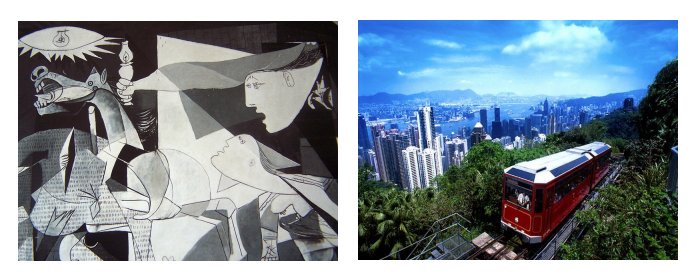
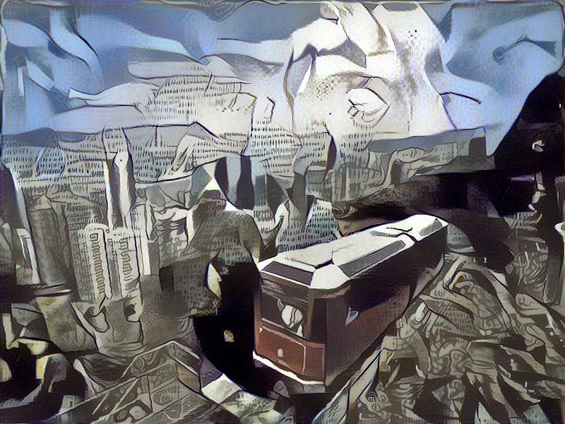
The idea is to use the filter responses from different layers of a convolutional network to build the style. Using filter responses from different layers (ranging from lower to higher) captures from low level details (strokes, points, corners) to high level details (patterns, objects, etc) which we will used to perturb the content image, which gives the final “painted” image:

Using Guernica’s style painting and Hong Kong’s Peak Tram to yield this:

Code

We need to define come constants for the image. If you want to use another style or image, just modify the STYLE_IMAGE or CONTENT_IMAGE. For this notebook, I hardcoded the image width to be 800 x 600, but you can easily modify the code to accommodate different sizes.

1
2
3
4
5
6
7
8
9
10
11
12
13
14
# Constants for the image input and output.
###############################################################################

# Output folder for the images.
OUTPUT_DIR = 'output/'
# Style image to use.
STYLE_IMAGE = 'images/guernica.jpg'
# Content image to use.
CONTENT_IMAGE = 'images/hongkong.jpg'
# Image dimensions constants. 
IMAGE_WIDTH = 800
IMAGE_HEIGHT = 600
COLOR_CHANNELS = 3

Now we define some constants which is related to the algorithm. Given that the style image and the content image remains the same, these can be tweaked to achieve different outcomes. Comments are added before each constant.

1
2
3
4
5
6
7
8
9
10
11
12
13
14
15
16
17
18
19
20
21
# Algorithm constants
###############################################################################
# Noise ratio. Percentage of weight of the noise for intermixing with the
# content image.
NOISE_RATIO = 0.6
# Constant to put more emphasis on content loss.
BETA = 5
# Constant to put more emphasis on style loss.
ALPHA = 100
# Path to the deep learning model. This is more than 500MB so will not be
# included in the repository, but available to download at the model Zoo:
# Link: https://github.com/BVLC/caffe/wiki/Model-Zoo
#
# Pick the VGG 19-layer model by from the paper "Very Deep Convolutional 
# Networks for Large-Scale Image Recognition".
VGG_MODEL = 'imagenet-vgg-verydeep-19.mat'
# The mean to subtract from the input to the VGG model. This is the mean that
# when the VGG was used to train. Minor changes to this will make a lot of
# difference to the performance of model.
MEAN_VALUES = np.array([123.68, 116.779, 103.939]).reshape((1,1,1,3))

Now we need to define the model that “paints” the image. Rather than training a completely new model from scratch, we will use a pre-trained model to achieve our purpose - called “transfer learning”.

We will use the VGG19 model. You can download the VGG19 model from here. The comments below describes the dimensions of the VGG19 model. We will replace the max pooling layers with average pooling layers as the paper suggests, and discard all fully connected layers.

1
2
3
4
5
6
7
8
9
10
11
12
13
14
15
16
17
18
19
20
21
22
23
24
25
26
27
28
29
30
31
32
33
34
35
36
37
38
39
40
41
42
43
44
45
46
47
48
49
50
51
52
53
54
55
56
57
58
59
60
61
62
63
64
65
66
67
68
69
70
71
72
73
74
75
76
77
78
79
80
81
82
83
84
85
86
87
88
89
90
91
92
93
94
95
96
97
98
99
100
101
102
103
104
105
106
107
108
109
110
111
112
113
114
115
116
117
118
119
120
def load_vgg_model(path):
 """
 Returns a model for the purpose of 'painting' the picture.
 Takes only the convolution layer weights and wrap using the TensorFlow
 Conv2d, Relu and AveragePooling layer. VGG actually uses maxpool but
 the paper indicates that using AveragePooling yields better results.
 The last few fully connected layers are not used.
 Here is the detailed configuration of the VGG model:
 0 is conv1_1 (3, 3, 3, 64)
 1 is relu
 2 is conv1_2 (3, 3, 64, 64)
 3 is relu 
 4 is maxpool
 5 is conv2_1 (3, 3, 64, 128)
 6 is relu
 7 is conv2_2 (3, 3, 128, 128)
 8 is relu
 9 is maxpool
 10 is conv3_1 (3, 3, 128, 256)
 11 is relu
 12 is conv3_2 (3, 3, 256, 256)
 13 is relu
 14 is conv3_3 (3, 3, 256, 256)
 15 is relu
 16 is conv3_4 (3, 3, 256, 256)
 17 is relu
 18 is maxpool
 19 is conv4_1 (3, 3, 256, 512)
 20 is relu
 21 is conv4_2 (3, 3, 512, 512)
 22 is relu
 23 is conv4_3 (3, 3, 512, 512)
 24 is relu
 25 is conv4_4 (3, 3, 512, 512)
 26 is relu
 27 is maxpool
 28 is conv5_1 (3, 3, 512, 512)
 29 is relu
 30 is conv5_2 (3, 3, 512, 512)
 31 is relu
 32 is conv5_3 (3, 3, 512, 512)
 33 is relu
 34 is conv5_4 (3, 3, 512, 512)
 35 is relu
 36 is maxpool
 37 is fullyconnected (7, 7, 512, 4096)
 38 is relu
 39 is fullyconnected (1, 1, 4096, 4096)
 40 is relu
 41 is fullyconnected (1, 1, 4096, 1000)
 42 is softmax
 """
 vgg = scipy.io.loadmat(path)

 vgg_layers = vgg['layers']
 def _weights(layer, expected_layer_name):
 Return the weights and bias from the VGG model for a given layer.
 """
 W = vgg_layers[0][layer][0][0][0][0][0]
 b = vgg_layers[0][layer][0][0][0][0][1]
 layer_name = vgg_layers[0][layer][0][0][-2]
 assert layer_name == expected_layer_name
 return W, b

 def _relu(conv2d_layer):
 """
 Return the RELU function wrapped over a TensorFlow layer. Expects a
 Conv2d layer input.
 """
 return tf.nn.relu(conv2d_layer)

 def _conv2d(prev_layer, layer, layer_name):
 """
 Return the Conv2D layer using the weights, biases from the VGG
 model at 'layer'.
 """
 W, b = _weights(layer, layer_name)
 W = tf.constant(W)
 b = tf.constant(np.reshape(b, (b.size)))
 return tf.nn.conv2d(
 prev_layer, filter=W, strides=[1, 1, 1, 1], padding='SAME') + b

 def _conv2d_relu(prev_layer, layer, layer_name):
 """
 Return the Conv2D + RELU layer using the weights, biases from the VGG
 model at 'layer'.
 """
 return _relu(_conv2d(prev_layer, layer, layer_name))

 def _avgpool(prev_layer):
 Return the AveragePooling layer.
 """
 return tf.nn.avg_pool(prev_layer, ksize=[1, 2, 2, 1], strides=[1, 2, 2, 1], padding='SAME')

 # Constructs the graph model.
 graph = {}
 graph['input'] = tf.Variable(np.zeros((1, IMAGE_HEIGHT, IMAGE_WIDTH, COLOR_CHANNELS)), dtype = 'float32')
 graph['conv1_1'] = _conv2d_relu(graph['input'], 0, 'conv1_1')
 graph['conv1_2'] = _conv2d_relu(graph['conv1_1'], 2, 'conv1_2')
 graph['avgpool1'] = _avgpool(graph['conv1_2'])
 graph['conv2_1'] = _conv2d_relu(graph['avgpool1'], 5, 'conv2_1')
 graph['conv2_2'] = _conv2d_relu(graph['conv2_1'], 7, 'conv2_2')
 graph['avgpool2'] = _avgpool(graph['conv2_2'])
 graph['conv3_1'] = _conv2d_relu(graph['avgpool2'], 10, 'conv3_1')
 graph['conv3_2'] = _conv2d_relu(graph['conv3_1'], 12, 'conv3_2')
 graph['conv3_3'] = _conv2d_relu(graph['conv3_2'], 14, 'conv3_3')
 graph['conv3_4'] = _conv2d_relu(graph['conv3_3'], 16, 'conv3_4')
 graph['avgpool3'] = _avgpool(graph['conv3_4'])
 graph['conv4_1'] = _conv2d_relu(graph['avgpool3'], 19, 'conv4_1')
 graph['conv4_2'] = _conv2d_relu(graph['conv4_1'], 21, 'conv4_2')
 graph['conv4_3'] = _conv2d_relu(graph['conv4_2'], 23, 'conv4_3')
 graph['conv4_4'] = _conv2d_relu(graph['conv4_3'], 25, 'conv4_4')
 graph['avgpool4'] = _avgpool(graph['conv4_4'])
 graph['conv5_1'] = _conv2d_relu(graph['avgpool4'], 28, 'conv5_1')
 graph['conv5_2'] = _conv2d_relu(graph['conv5_1'], 30, 'conv5_2')
 graph['conv5_3'] = _conv2d_relu(graph['conv5_2'], 32, 'conv5_3')
 graph['conv5_4'] = _conv2d_relu(graph['conv5_3'], 34, 'conv5_4')
 graph['avgpool5'] = _avgpool(graph['conv5_4'])
 return graph

Define the equation (1) from the paper to model the content loss. We are only concerned with the “conv4_2” layer of the model.

1
2
3
4
5
6
7
8
9
10
11
12
13
14
15
16
17
def content_loss_func(sess, model):
 Content loss function as defined in the paper.
 """
 def _content_loss(p, x):
 # N is the number of filters (at layer l).
 N = p.shape[3]
 # M is the height times the width of the feature map (at layer l).
 M = p.shape[1] * p.shape[2]
 # Interestingly, the paper uses this form instead:
 # 0.5 * tf.reduce_sum(tf.pow(x - p, 2)) 
 #
 # But this form is very slow in "painting" and thus could be missing
 # out some constants (from what I see in other source code), so I'll
 # replicate the same normalization constant as used in style loss.
 return (1 / (4 * N * M)) * tf.reduce_sum(tf.pow(x - p, 2))
 return _content_loss(sess.run(model['conv4_2']), model['conv4_2'])

Define the equation (5) from the paper to model the style loss. The style loss is a multi-scale representation. It is a summation from conv1_1 (lower layer) to conv5_1 (higher layer). Intuitively, the style loss across multiple layers captures lower level features (hard strokes, points, etc) to higher level features (styles, patterns, even objects).

You can tune the weights in the STYLE_LAYERS to yield very different results. See the Bonus part at the bottom for more illustrations.

1
2
3
4
5
6
7
8
9
10
11
12
13
14
15
16
17
18
19
20
21
22
23
24
25
26
27
28
29
30
31
32
33
34
35
36
37
38
39
40
41
# Layers to use. We will use these layers as advised in the paper.
# To have softer featur
es, increase the weight of the higher layers
# (conv5_1) and decrease the weight of the lower layers (conv1_1).
# To have harder features, decrease the weight of the higher layers
# (conv5_1) and increase the weight of the lower layers (conv1_1).
STYLE_LAYERS = [
 ('conv1_1', 0.5),
 ('conv2_1', 1.0),
 ('conv3_1', 1.5),
 ('conv4_1', 3.0),
 ('conv5_1', 4.0),
]

def style_loss_func(sess, model):
 Style loss function as defined in the paper.
 def _gram_matrix(F, N, M):
 The gram matrix G.
 """
 Ft = tf.reshape(F, (M, N))
 return tf.matmul(tf.transpose(Ft), Ft)

 def _style_loss(a, x):
 The style loss calculation.
 """
 # N is the number of filters (at layer l).
 N = a.shape[3]
 # M is the height times the width of the feature map (at layer l).
 M = a.shape[1] * a.shape[2]
 # A is the style representation of the original image (at layer l).
 A = _gram_matrix(a, N, M)
 # G is the style representation of the generated image (at layer l).
 G = _gram_matrix(x, N, M)
 result = (1 / (4 * N**2 * M**2)) * tf.reduce_sum(tf.pow(G - A, 2))
 return result

 E = [_style_loss(sess.run(model[layer_name]), model[layer_name]) for layer_name, _ in STYLE_LAYERS]
 W = [w for _, w in STYLE_LAYERS]
 loss = sum([W[l] * E[l] for l in range(len(STYLE_LAYERS))])
 return loss

Define the rest of the auxiliary functions.

1
2
3
4
5
6
7
8
9
10
11
12
13
14
15
16
17
18
19
20
21
22
23
24
25
26
27
28
def generate_noise_image(content_image, noise_ratio = NOISE_RATIO):
 Returns a noise image intermixed with the content image at a certain ratio.
 """
 noise_image = np.random.uniform(
 -20, 20,
 (1, IMAGE_HEIGHT, IMAGE_WIDTH, COLOR_CHANNELS)).astype('float32')
 # White noise image from the content representation. Take a weighted average
 # of the values
 input_image = noise_image * noise_ratio + content_image * (1 - noise_ratio)
 return input_image

def load_image(path):
 image = scipy.misc.imread(path)
 # Resize the image for convnet input, there is no change but just
 # add an extra dimension.
 image = np.reshape(image, ((1,) + image.shape))
 # Input to the VGG model expects the mean to be subtracted.
 image = image - MEAN_VALUES
 return image

def save_image(path, image):
 # Output should add back the mean.
 image = image + MEAN_VALUES
 # Get rid of the first useless dimension, what remains is the image.
 image = image[0]
 image = np.clip(image, 0, 255).astype('uint8')
 scipy.misc.imsave(path, image)

Create an TensorFlow session.

1
2
sess = tf.InteractiveSession()

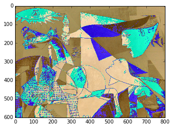
Now we load the content image “Hong Kong”. The model expects an image with MEAN_VALUES subtracted to function correctly. “load_image” already handles this. The showed image will look funny.

1
2
3
4
content_image = load_image(CONTENT_IMAGE)
imshow(content_image[0])


<matplotlib.image.AxesImage at 0x7fd90c111240>

1
2
3
4
5
6

![](http://www.chioka.in/wp-content/uploads/2016/05/output_19_1.png)


Now we load the style image using Guernica. Similarly, the color will look distorted but that’s what the model needs:

style_image = load_image(STYLE_IMAGE) imshow(style_image[0])

1
2
<matplotlib.image.AxesImage at 0x7fd90c041780>

Build the model now.

1
2
3
4
model = load_vgg_model(VGG_MODEL)
print(model)


{‘conv1_1’: <tf.Tensor ‘Relu:0’ shape=(1, 600, 800, 64) dtype=float32>, ‘conv5_4’: <tf.Tensor ‘Relu_15:0’ shape=(1, 38, 50, 512) dtype=float32>, ‘conv2_2’: <tf.Tensor ‘Relu_3:0’ shape=(1, 300, 400, 128) dtype=float32>, ‘conv4_2’: <tf.Tensor ‘Relu_9:0’ shape=(1, 75, 100, 512) dtype=float32>, ‘avgpool1’: <tf.Tensor ‘AvgPool:0’ shape=(1, 300, 400, 64) dtype=float32>, ‘input’: <tensorflow.python.ops.variables.Variable object at 0x7fd90c0536a0>, ‘conv1_2’: <tf.Tensor ‘Relu_1:0’ shape=(1, 600, 800, 64) dtype=float32>, ‘conv3_3’: <tf.Tensor ‘Relu_6:0’ shape=(1, 150, 200, 256) dtype=float32>, ‘conv3_2’: <tf.Tensor ‘Relu_5:0’ shape=(1, 150, 200, 256) dtype=float32>, ‘avgpool3’: <tf.Tensor ‘AvgPool_2:0’ shape=(1, 75, 100, 256) dtype=float32>, ‘avgpool2’: <tf.Tensor ‘AvgPool_1:0’ shape=(1, 150, 200, 128) dtype=float32>, ‘conv3_1’: <tf.Tensor ‘Relu_4:0’ shape=(1, 150, 200, 256) dtype=float32>, ‘conv4_3’: <tf.Tensor ‘Relu_10:0’ shape=(1, 75, 100, 512) dtype=float32>, ‘conv5_3’: <tf.Tensor ‘Relu_14:0’ shape=(1, 38, 50, 512) dtype=float32>, ‘conv2_1’: <tf.Tensor ‘Relu_2:0’ shape=(1, 300, 400, 128) dtype=float32>, ‘avgpool4’: <tf.Tensor ‘AvgPool_3:0’ shape=(1, 38, 50, 512) dtype=float32>, ‘conv4_4’: <tf.Tensor ‘Relu_11:0’ shape=(1, 75, 100, 512) dtype=float32>, ‘conv4_1’: <tf.Tensor ‘Relu_8:0’ shape=(1, 75, 100, 512) dtype=float32>, ‘conv3_4’: <tf.Tensor ‘Relu_7:0’ shape=(1, 150, 200, 256) dtype=float32>, ‘conv5_2’: <tf.Tensor ‘Relu_13:0’ shape=(1, 38, 50, 512) dtype=float32>, ‘avgpool5’: <tf.Tensor ‘AvgPool_4:0’ shape=(1, 19, 25, 512) dtype=float32>, ‘conv5_1’: <tf.Tensor ‘Relu_12:0’ shape=(1, 38, 50, 512) dtype=float32>}

1
2
3
4
5
6
# Generate the white noise and content presentation mixed image
# which will be the basis for the algorithm to "paint".
input_image = generate_noise_image(content_image)
imshow(input_image[0])


<matplotlib.image.AxesImage at 0x7fd9047c0c18>

1
2
3
4

![](http://www.chioka.in/wp-content/uploads/2016/05/output_24_1.png)


sess.run(tf.initialize_all_variables())

1
2
3
4
5
# Construct content_loss using content_image.
sess.run(model['input'].assign(content_image))
content_loss = content_loss_func(sess, model)


Construct style_loss using style_image.

sess.run(model[‘input’].assign(style_image)) style_loss = style_loss_func(sess, model)

1
2
3
4
# Instantiate equation 7 of the paper.
total_loss = BETA * content_loss + ALPHA * style_loss


From the paper: jointly minimize the distance of a white noise image

from the content representation of the photograph in one layer of

the neywork and the style representation of the painting in a number

of layers of the CNN.

#

The content is built from one layer, while the style is from five

layers. Then we minimize the total_loss, which is the equation 7.

optimizer = tf.train.AdamOptimizer(2.0) train_step = optimizer.minimize(total_loss)

1
2
3
4
sess.run(tf.initialize_all_variables())
sess.run(model['input'].assign(input_image))


array([[[[-38.80082321, 2.36044788, 53.06735229], [-36.208992 , -8.92279434, 52.68152237], [-44.56254196, 2.56879926, 42.36888885], …, [-21.99048233, 6.0762639 , 39.36758041], [-35.85998535, -3.56352782, 44.86796951], [-42.85255051, -6.79411459, 52.11099625]],

[[-35.10824203, -10.4971714 , 38.89696884], [-37.86809921, -5.79524469, 39.4394722 ], [-27.90998077, 1.6464256 , 52.97366714], …, [-44.19208527, -13.92263412, 36.78689194], [-39.15240097, -2.04686642, 49.2306633 ], [-35.7723732 , -12.24501419, 44.17518997]],

[[-43.50813675, -7.48234081, 48.60139465], [-34.67430878, -7.62575102, 36.58321762], [-34.54434586, -15.8774004 , 38.89173126], …, [-32.95817947, -3.49402404, 38.15805054], [-25.93852997, -14.92780209, 49.86390686], [-44.59893417, -8.43691158, 41.84837723]],

…, [[-55.29382324, -57.94036865, -47.33403397], [-47.22367859, -47.09892654, -43.59551239], [-58.79758072, -43.68718719, -52.4673996 ], …, [-51.44662857, -39.4832077 , -46.86067581], [-37.68956375, -39.0056076 , -41.35289383], [-46.67458725, -46.07319641, -42.1647644 ]],

[[-40.65664291, -39.99607086, -50.46044159], [-39.84476471, -47.29466629, -42.65992355], [-46.70065689, -56.47098923, -33.3544693 ], …, [-57.43079376, -49.95788956, -34.21024704], [-42.41124344, -44.70735168, -40.68310928], [-48.97134781, -41.0301857 , -48.75336456]],

[[-46.85499191, -52.87174606, -42.00823975], [-52.52578354, -50.29984665, -49.69490814], [-54.52784348, -39.16690063, -42.48467255], …, [-56.66353226, -34.45768356, -31.35286331], [-42.40987396, -31.03708076, -38.9402504 ], [-44.44059753, -45.45861435, -38.15160751]]]], dtype=float32)

1
2
3
4
5

Change the ITERATIONS to run 5000 iterations if you can wait. It takes about 90 minutes to run 5000 iterations. So in this notebook I will just run 1000 iterations so no one waits too long.

Run the model which outputs the painted image every 100 iterations. The final image is what we need:

Number of iterations to run.

ITERATIONS = 1000 # The art.py uses 5000 iterations, and yields far more appealing results. If you can wait, use 5000.

1
2
3
4
5
6
7
8
9
10
11
12
13
14
15
16
17
18
sess.run(tf.initialize_all_variables())
sess.run(model['input'].assign(input_image))
for it in range(ITERATIONS):
 sess.run(train_step)
 if it%100 == 0:
 # Print every 100 iteration.
 mixed_image = sess.run(model['input'])
 print('Iteration %d' % (it))
 print('sum : ', sess.run(tf.reduce_sum(mixed_image)))
 print('cost: ', sess.run(total_loss))

 if not os.path.exists(OUTPUT_DIR):
 os.mkdir(OUTPUT_DIR)

 filename = 'output/%d.png' % (it)
 save_image(filename, mixed_image)


Iteration 0 sum : -4.70464e+06 cost: 7.69395e+10 Iteration 100 sum : -2.9841e+06 cost: 3.54706e+09 Iteration 200 sum : -2.43492e+06 cost: 1.39629e+09 Iteration 300 sum : -1.32645e+06 cost: 7.6313e+08 Iteration 400 sum : -39769.0 cost: 4.84996e+08 Iteration 500 sum : 1.18856e+06 cost: 3.54245e+08 Iteration 600 sum : 2.1015e+06 cost: 3.0398e+08 Iteration 700 sum : 3.1431e+06 cost: 2.04405e+08 Iteration 800 sum : 4.07144e+06 cost: 1.6504e+08 Iteration 900 sum : 4.9075e+06 cost: 1.34236e+08
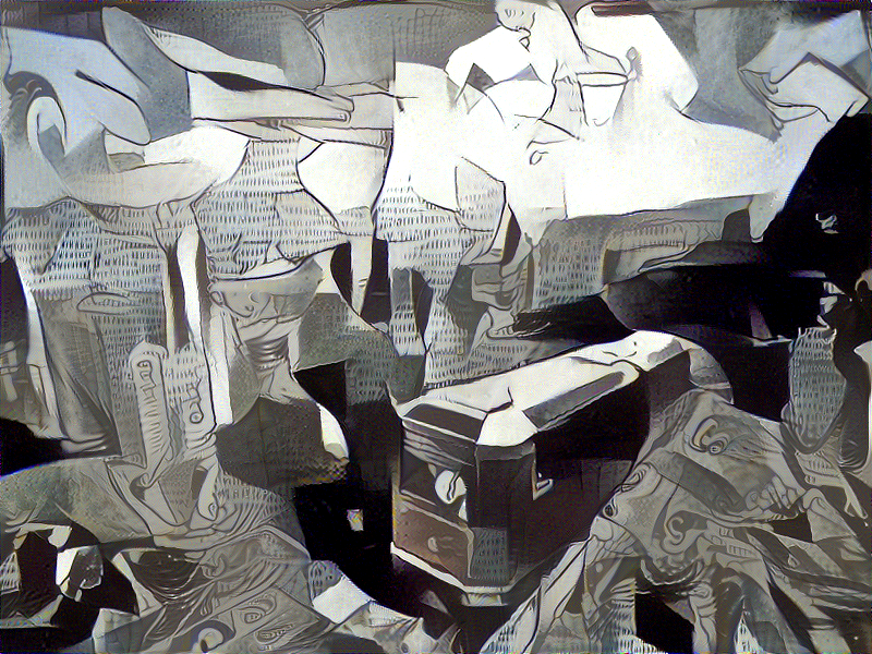
1
2
save_image('output/art.jpg', mixed_image)

This is our final art for 1000 iterations. It is different the one above which I have ran for 5000 iterations. However, you can certainly generate your own painting now.

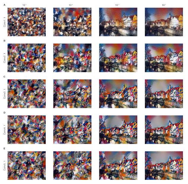
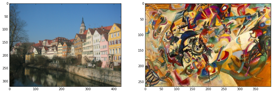
Bonus : Style Weights Illustrated

By tweaking the weights in the style layer loss function, you may be able to put more emphasis on lower level features or higher level features yielding quite a different painting. Here is what is shown in the original paper. Using this picture “Composition” as style and “Tubingen” as content:

1
2
3
4
5
6
7
8
9
from PIL import Image
fig = plt.figure()
fig.set_size_inches(30, 10.5)
fig_1 = fig.add_subplot(2,1,1)
fig_1.imshow(np.asarray(Image.open('article/composition.jpg')))
fig_1 = fig.add_subplot(2,2,1)
fig_1.imshow(np.asarray(Image.open('article/tubingen.jpg')))


<matplotlib.image.AxesImage at 0x7f092e9add30>

```

The upper leftmost corner indicates a picture that puts more weight on the lower level features, and the resulting image is completely deformed and only included low level features. The lower right uses mostly the higher level features and less lower level features, and the image is less deformed and quite appealing, which is what this notebook is doing as well. Feel free to play with the weights above.