The need for anomaly and change detection will pop up in almost any data driven system or quality monitoring application. Typically, there a set of metrics that need to be monitored and an alert raised if the values deviate from the expected. Depending on the task at hand, this can happen at individual datapoint level (anomaly detection) or population level where we want to know if the underlying distribution changes or not (change detection).
The latter is most commonly tackled by the most straightforward: calculating some point estimates, typically the mean or median and track these. This could be time based such as calculating the daily mean, or be based on some unit of “work done” such as for batches in a production line or versions in software product. The calculated point estimates can be displayed on dashboards to be checked visually or a delta computed between consequtive numbers, which can be compared against some pre-defined threshold to see if an alarm should be raised.
The problem with such point estimates is that they don’t necessarily capture the change in the underlying distribution of the tracked measure well. A change in the distribution can be signficicant while the mean or the median remains unchanged.
In cases when change needs to be detected, measuring it directly on the distribution is typically a much better option.
Histogram intersection calculates the similarity of two discretized probability distributions (histograms), with possible value of the intersection lying between 0 (no overlap) and 1 (identical distributions). Given bin edges and two normalized histogram, it can be calculated by
For example for the two distributions (\mathcal{N}(2,1)) and (\mathcal{N}(3,1.5)), the intersection is ~0.66, easy to represent graphically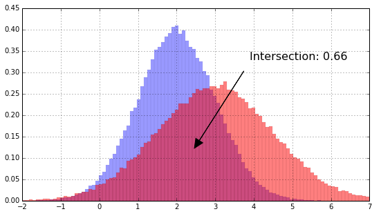
Histogram intersection has a few extra benefits:
- It works equally well on categorical data, where we can use category frequencies to compute the intersection
Dealing with null values comes for free, simply by making nulls part of the distribution: if there is an increase in nulls, it changes the intersection, even if non-null values will continue to be distributed the same way. In contrast, when tracking point estimates such as the mean, null value checks need to be explicitly added as an additional item to track.
As always, there are some caveats. One issue is that the intersection depends on how the bins have been selected. This becomes an issue especially for long tailed distributions. For example for the lognormal distribution, with same (\mu) and (\sigma) as above, the histogram might look something like the following, with practically all density concentrated in the first bin. Calculating the intersection on that would clearly give very misleading results.
This can be tackled by either moving the histogram to log-scale, or simply by clipping the long tail to use it as an approximtion. For this particular examples clipping gives the same result as the “true” intersection calculted in log scale.

Kullback-Leibler divergence and statistical tests
Two methods often recommended for detecting change in distribution are Kullback-Leibler divergence and statistical tests, for example a chi-squared test which could be used both on categorical data and a histogram of continous data. Both of the methods have significant drawbacks however.
Kullback-Leibler divergence is measured in bits and unlike histogram intersection, does not lie in a given range. This makes comparison on two different dataset difficult. Secondly, it is only defined when zeroes in the distributions lie in the same bins. Ths can be overcome by transferrning some of the probability mass to locations with zero probability, however, this is another extra complexity that needs to be handled. Finally, KL divergence is not a true metric, i.e. it does not obey triangle inequality, and is non-symmetric, i.e. in general, when comparing two different distributions (P) and (Q), (KL(P,Q) \neq KL(Q,P)).
Using a statistical test, for example a chi-squared test might seem like a good option, since it gives you a p-value you can use to estimate how likely it is that the distribution has changed. The problem is that the p-value of a test is a function of the size of the data, so we can obtain tiny p-values with very small differences in the distributions. In the following, we are comparing (\mathcal{N}(0,1)) and (\mathcal{N}(0.005,1)) in the first plot, and (\mathcal{N}(0,1)) and (\mathcal{N}(1,1)) in the second plot.
In both cases, we have tiny p-values, in fact it is even smaller for the first plot. From practical point of view, the change in the first case is likely irrelevant, since the absolute change is so small.
A chi-squared test can of course still be very useful and complement the histogram intersection, by letting us know if the amount of data is small enough that measuring the intersection likely won’t give meaningful results.
Beyond histogram intersection
One drawback of histogram intersection is that it does not consider distances between bins, which can be important in case of ordinal data.
For example, consider the following plot with three different histograms. Histogram intersection between histograms 1 and 2, and 1 and 3 are the same. However, assuming it is ordinal data, we might want to say that histgorams 1 and 2 are actually more similar to each other, since the changed bins are closer to each other than the change between 1 and 3.
There are various methods to take this into account, the most well known being earth mover’s distance. There is a nice overview of these methods here.