This is straightforward. Certain types of input create certain types of hidden layers. Certain types of hidden layers create certain types of output layers. It’s kindof a closed system. Memory changes this. Memory means that the hidden layer is a combination of your input data at the current timestep and the hidden layer of the previous timestep.
Why the hidden layer? Well, we could technically do this.
However, we’d be missing out. I encourage you to sit and consider the difference between these two information flows. For a little helpful hint, consider how this plays out. Here, we have 4 timesteps of a recurrent neural network pulling information from the previous hidden layer.
And here, we have 4 timesteps of a recurrent neural network pulling information from the previous input layer
Maybe, if I colored things a bit, it would become more clear. Again, 4 timesteps with hidden layer recurrence:
…. and 4 timesteps with input layer recurrence….
Focus on the last hidden layer (4th line). In the hidden layer recurrence, we see a presence of every input seen so far. In the input layer recurrence, it’s exclusively defined by the current and previous inputs. This is why we model hidden recurrence. Hidden recurrence learns what to remember whereas input recurrence is hard wired to just remember the immediately previous datapoint.
Now compare and contrast these two approaches with the backwards alphabet and middle-of-song exercises. The hidden layer is constantly changing as it gets more inputs. Furthermore, the only way that we could reach these hidden states is with the correct sequence of inputs. Now the money statement, the output is deterministic given the hidden layer, and the hidden layer is only reachable with the right sequence of inputs. Sound familiar?
What’s the practical difference? Let’s say we were trying to predict the next word in a song given the previous. The “input layer recurrence” would break down if the song accidentally had the same sequence of two words in multiple places. Think about it, if the song had the statements “I love you”, and “I love carrots”, and the network was trying to predict the next word, how would it know what follows “I love”? It could be carrots. It could be you. The network REALLY needs to know more about what part of the song its in. However, the “hidden layer recurrence” doesn’t break down in this way. It subtely remembers everything it saw (with memories becoming more subtle as it they fade into the past). To see this in action, check out this.
stop and make sure this feels comfortable in your mindPart 2: RNN - Neural Network Memory
Now that we have the intuition, let’s dive down a layer (ba dum bump…). As described in the backpropagation post, our input layer to the neural network is determined by our input dataset. Each row of input data is used to generate the hidden layer (via forward propagation). Each hidden layer is then used to populate the output layer (assuming only 1 hidden layer). As we just saw, memory means that the hidden layer is a combination of the input data and the previous hidden layer. How is this done? Well, much like every other propagation in neural networks, it’s done with a matrix. This matrix defines the relationship between the previous hidden layer and the current one.
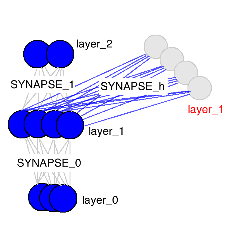
Big thing to take from this picture, there are only three weight matrices. Two of them should be very familiar (same names too). SYNAPSE_0 propagates the input data to the hidden layer. SYNAPSE_1 propagates the hidden layer to the output data. The new matrix (SYNAPSE_h….the recurrent one), propagates from the hidden layer (layer_1) to the hidden layer at the next timestep (still layer_1).
stop and make sure this feels comfortable in your mind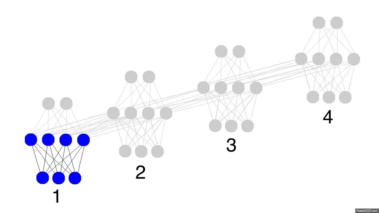
The gif above reflects the magic of recurrent networks, and several very, very important properties. It depicts 4 timesteps. The first is exclusively influenced by the input data. The second one is a mixture of the first and second inputs. This continues on. You should recognize that, in some way, network 4 is “full”. Presumably, timestep 5 would have to choose which memories to keep and which ones to overwrite. This is very real. It’s the notion of memory “capacity”. As you might expect, bigger layers can hold more memories for a longer period of time. Also, this is when the network learns to forget irrelevant memories and remember important memories. What significant thing do you notice in timestep 3? Why is there more green in the hidden layer than the other colors?
Also notice that the hidden layer is the barrier between the input and the output. In reality, the output is no longer a pure function of the input. The input is just changing what’s in the memory, and the output is exclusively based on the memory. Another interesting takeaway. If there was no input at timesteps 2,3,and 4, the hidden layer would still change from timestep to timestep.
Part 3: Backpropagation Through Time:
So, how do recurrent neural networks learn? Check out this graphic. Black is the prediction, errors are bright yellow, derivatives are mustard colored.

They learn by fully propagating forward from 1 to 4 (through an entire sequence of arbitrary length), and then backpropagating all the derivatives from 4 back to 1. You can also pretend that it’s just a funny shaped normal neural network, except that we’re re-using the same weights (synapses 0,1,and h) in their respective places. Other than that, it’s normal backpropagation.
Part 4: Our Toy Code
We’re going to be using a recurrent neural network to model binary addition. Do you see the sequence below? What do the colored ones in squares at the top signify?
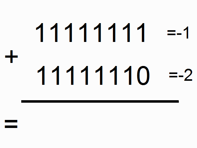
The colorful 1s in boxes at the top signify the “carry bit”. They “carry the one” when the sum overfows at each place. This is the tiny bit of memory that we’re going to teach our neural network how to model. It’s going to “carry the one” when the sum requires it. (click here to learn about when this happens)
So, binary addition moves from right to left, where we try to predict the number beneath the line given the numbers above the line. We want the neural network to move along the binary sequences and remember when it has carried the 1 and when it hasn’t, so that it can make the correct prediction. Don’t get too caught up in the problem. The network actually doesn’t care too much. Just recognize that we’re going to have two inputs at each time step, (either a one or a zero from each number begin added). These two inputs will be propagated to the hidden layer, which will have to remember whether or not we carry. The prediction will take all of this information into account to predict the correct bit at the given position (time step).
Lines 0-2: Importing our dependencies and seeding the random number generator. We will only use numpy and copy. Numpy is for matrix algebra. Copy is to copy things.
Lines 4-11: Our nonlinearity and derivative. For details, please read this Neural Network Tutorial
Line 15: We’re going to create a lookup table that maps from an integer to its binary representation. The binary representations will be our input and output data for each math problem we try to get the network to solve. This lookup table will be very helpful in converting from integers to bit strings.
Line 16: This is where I set the maximum length of the binary numbers we’ll be adding. If I’ve done everything right, you can adjust this to add potentially very large numbers.
Line 18: This computes the largest number that is possible to represent with the binary length we chose
Line 19: This is a lookup table that maps from an integer to its binary representation. We copy it into the int2binary. This is kindof un-ncessary but I thought it made things more obvious looking.
Line 26: This is our learning rate.
Line 27: We are adding two numbers together, so we’ll be feeding in two-bit strings one character at the time each. Thus, we need to have two inputs to the network (one for each of the numbers being added).
Line 28: This is the size of the hidden layer that will be storing our carry bit. Notice that it is way larger than it theoretically needs to be. Play with this and see how it affects the speed of convergence. Do larger hidden dimensions make things train faster or slower? More iterations or fewer?
Line 29: Well, we’re only predicting the sum, which is one number. Thus, we only need one output
Line 33: This is the matrix of weights that connects our input layer and our hidden layer. Thus, it has “input_dim” rows and “hidden_dim” columns. (2 x 16 unless you change it). If you forgot what it does, look for it in the pictures in Part 2 of this blogpost.
Line 34: This is the matrix of weights that connects the hidden layer to the output layer. Thus, it has “hidden_dim” rows and “output_dim” columns. (16 x 1 unless you change it). If you forgot what it does, look for it in the pictures in Part 2 of this blogpost.
Line 35: This is the matrix of weights that connects the hidden layer in the previous time-step to the hidden layer in the current timestep. It also connects the hidden layer in the current timestep to the hidden layer in the next timestep (we keep using it). Thus, it has the dimensionality of “hidden_dim” rows and “hidden_dim” columns. (16 x 16 unless you change it). If you forgot what it does, look for it in the pictures in Part 2 of this blogpost.
Line 37 - 39: These store the weight updates that we would like to make for each of the weight matrices. After we’ve accumulated several weight updates, we’ll actually update the matrices. More on this later.
Line 42: We’re iterating over 100,000 training examples
Line 45: We’re going to generate a random addition problem. So, we’re initializing an integer randomly between 0 and half of the largest value we can represent. If we allowed the network to represent more than this, than adding two number could theoretically overflow (be a bigger number than we have bits to represent). Thus, we only add numbers that are less than half of the largest number we can represent.
Line 46: We lookup the binary form for “a_int” and store it in “a”
Line 48: Same thing as line 45, just getting another random number.
Line 49: Same thing as line 46, looking up the binary representation.
Line 52: We’re computing what the correct answer should be for this addition
Line 53: Converting the true answer to its binary representation
Line 56: Initializing an empty binary array where we’ll store the neural network’s predictions (so we can see it at the end). You could get around doing this if you want…but i thought it made things more intuitive
Line 58: Resetting the error measure (which we use as a means to track convergence… see my tutorial on backpropagation and gradient descent to learn more about this)
Lines 60-61: These two lists will keep track of the layer 2 derivatives and layer 1 values at each time step.
Line 62: Time step zero has no previous hidden layer, so we initialize one that’s off.
Line 65: This for loop iterates through the binary representation
Line 68: X is the same as “layer_0” in the pictures. X is a list of 2 numbers, one from a and one from b. It’s indexed according to the “position” variable, but we index it in such a way that it goes from right to left. So, when position == 0, this is the farhest bit to the right in “a” and the farthest bit to the right in “b”. When position equals 1, this shifts to the left one bit.
Line 69: Same indexing as line 62, but instead it’s the value of the correct answer (either a 1 or a 0)
Line 72: This is the magic!!! Make sure you understand this line!!! To construct the hidden layer, we first do two things. First, we propagate from the input to the hidden layer (np.dot(X,synapse_0)). Then, we propagate from the previous hidden layer to the current hidden layer (np.dot(prev_layer_1, synapse_h)). Then WE SUM THESE TWO VECTORS!!!!… and pass through the sigmoid function.
So, how do we combine the information from the previous hidden layer and the input? After each has been propagated through its various matrices (read: interpretations), we sum the information.
Line 75: This should look very familiar. It’s the same as previous tutorials. It propagates the hidden layer to the output to make a prediction
Line 78: Compute by how much the prediction missed
Line 79: We’re going to store the derivative (mustard orange in the graphic above) in a list, holding the derivative at each timestep.
Line 80: Calculate the sum of the absolute errors so that we have a scalar error (to track propagation). We’ll end up with a sum of the error at each binary position.
Line 83 Rounds the output (to a binary value, since it is between 0 and 1) and stores it in the designated slot of d.
Line 86 Copies the layer_1 value into an array so that at the next time step we can apply the hidden layer at the current one.
Line 90: So, we’ve done all the forward propagating for all the time steps, and we’ve computed the derivatives at the output layers and stored them in a list. Now we need to backpropagate, starting with the last timestep, backpropagating to the first
Line 92: Indexing the input data like we did before
Line 93: Selecting the current hidden layer from the list.
Line 94: Selecting the previous hidden layer from the list
Line 97: Selecting the current output error from the list
Line 99: this computes the current hidden layer error given the error at the hidden layer from the future and the error at the current output layer.
Line 102-104: Now that we have the derivatives backpropagated at this current time step, we can construct our weight updates (but not actually update the weights just yet). We don’t actually update our weight matrices until after we’ve fully backpropagated everything. Why? Well, we use the weight matrices for the backpropagation. Thus, we don’t want to go changing them yet until the actual backprop is done. See the backprop blog post for more details.
Line 109 - 115 Now that we’ve backpropped everything and created our weight updates. It’s time to update our weights (and empty the update variables).
Line 118 - end Just some nice logging to show progress