In past posts, I’ve described the geometry of artificial neural networks by thinking of the output from each neuron in the network as defining a probability density function on the space of input vectors. This is useful for understanding how a single neuron combines the outputs of other neurons to form a more complex shape. However, it’s often useful to think about how multiple neurons behave at the same time, particularly for networks that are defined by successive layers of neurons. For such networks – which turn out to be the vast majority of networks in practice – it’s useful to think about how the set of outputs from each layer determine the set of outputs of the next layer. In this post, I want to discuss how we can think about this in terms of linear transformations (via matrices) and how this idea leads to a tool called word embeddings, the most popular of which is probably word2vec.
First, recall that each neuron in a neural network has a number of inputs and a single output. The inputs come from either the features of an input vector, or from the outputs of other neurons. The neuron stores a weight for each input, and it calculates its output by multiplying each input value by a weight, adding up the products, adding a constant defined by another weight, then applying a fixed (non-linear) function to this value. One trains a neural network by modifying the weights on the inputs to each neuron so that the overall output is closer to what you want it to be.
Before we go any further, we’re going to split each of our neurons into two: We’ll call the first one a linear neuron – this will have the same inputs as the original neuron, but its output will simply add together the input-times-weight values, plus the constant weight. We’ll call the second neuron a non-linear neuron – it will take the output from the linear neuron as its only input, and apply the fixed non-linear function to it. So if we take a neural network and replace each of the original neurons by a linear neuron feeding into a non-linear neuron, we’ll get the same functionality as the original network.
An example of this is shown below. Adding arrow heads to show input/output made the picture too noisy, so you’ll have to pretend they’re all pointing to the right. In the top network, we have four input features feeding into a layer with two (standard) neurons, which in turn feed into a layer with three neurons, then a single neuron that combines their output to determine the output of the entire network. Below that, we have the same network after we’ve replaced each standard neuron with a linear neuron feeding into a non-linear neuron.
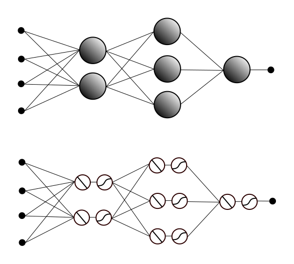
Notice that in the network after the split, the outputs from the non-linear neurons in a given row feed into the linear neurons in the next row. Let’s focus, for a moment, on the connections from the non-linear neurons in the first non-input row, to the linear neurons in the second non-input row.
The output values from the non-linear neurons define a vector that we’ll call V. The outputs from the linear neurons define another vector W. For each of the linear neurons in this row, there is one weight for each of the non-linear neurons in the previous row, so these weights define a vector with the same dimension/number of entries as V. In fact, we have one such vector for each of the linear neurons, and if we stack these vectors next to each other, we get a matrix, which we’ll call M.
So, lets just quickly review this: We have the vector V of outputs from the row of non-linear neurons and the vector W of outputs from the successive row of linear neurons. We calculate W by multiplying the entries in the vector V by certain entries in the matrix M and then adding them together in a certain way. Well, if you happen to remember how matrix multiplication works, and you think carefully about the way we’re multiplying and adding the neuron outputs and weights, they turn out to be the same thing. In other words, it just so happens that the vector W defined by the row of linear neurons is the result of (matrix) multiplication V *x *M. (I’m thinking of V as being horizontal and the vectors of the same dimension that make up M as vertical.)
We can think about this as a function/transformation from the space of all possible vectors V to the space of all possible vectors W. Under this interpretation, matrix multiplication defines a linear transformation: Every straight line in the first vector space will be sent to either a straight line or a point in the second space. (In particular, if the dimension of V is higher than that of W then a lot of lines will have to collapse down to points, but this can happen no matter what.) So there’s our geometric interpretation of the connections between the row of non-linear neurons and the next row of linear neurons: a linear transformation.
Oh, except there’s one small detail we forgot: Each neuron doesn’t just multiply and add the inputs from the previous row of neurons. It also adds in a constant weight. The set of constant weights define yet another vector C, with the same dimension as W, and adding in all the constant weights corresponds to adding C to the product V *x M.* But it turns out this isn’t such a big deal – it just means that we get an affine transformation instead of a linear transformation – straight lines still stay straight or collapse to points. However, the zero vector doesn’t necessarily go the the zero vector. So we still get a nice interpretation of the connections between the layers.
This brings up an interesting point about the importance of the non-linear neurons. If we were to remove the non-linear neurons and create a neural network entirely of linear neurons, then we could interpret the entire thing as a succession of linear transformations. So, for example, to calculate the output from the third layer, we would multiply the vector from the first layer by the matrix for the connections to the second layer, then multiply the resulting vector by the matrix for the connections from the second to the third layer. However, it turns out that combining linear transformations like this, which is equivalent to multiplying matrices, can only produce new linear or affine transformations. So we wouldn’t get anything with three layers that we couldn’t get with two. It’s the non-linear part of the neurons that allows neural networks to define arbitrarily complex probability distributions.
But lets return to the linear part. In addition to being a useful way to think about the layers in a neural network, it turns out these linear transformations also allow you to do some fun tricks such as transforming sparse data into dense data.
Sparse data in this context means data in which a typical data points has most of its features equal to zero, and its structure is determined more by which features are non-zero, than by what their values actually are. A good example of this is bag-of-words (BOW) vectors – the non-zero features reflect what the words in the “bag” are, and depending on the exact type of BOW, their actual values may or may not give you additional information such as word count.
The problem with this type of vector is that they’re floppy (That’s not a technical term.): Because there are so many dimensions, there’s a serious risk of overfitting, and the curse of dimensionality makes distances less meaningful. So to really understand the geometric structure of such data, we need a meaningful way to embed the data points into a lower-dimensional space.
It turns out one can do this by first trying to solve a different problem. Lets say you wanted to predict, for any given word, what other words are most likely to appear just before and just after it in a large corpus of text. In other words, given the word “apple” and the word “pie”, you want a model that tells you the probability, if you were to randomly select an occurrence of the word “apple” in the text, that “pie” would be one of the three words right before it or of the three words right after. (You can replace three with any number, but to simplify the discussion below, I’m going to stick with three.)
The most straightforward way to do this with a neural network is to have a row of inputs, with one input for each word, then a row of output neurons, one for each word, with every input feature attached to every output neuron. If you input a vector with value 1 for “apple” and value zero for everything else, you want the “pie” neuron to output the probability described above. We can achieve this by setting the weight on the edge from input “apple” to neuron “pie” to this probability (and we can calculate the probability directly by counting the number of occurrences in the corpus).
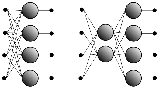
But this uses only sparse representations of the data, with one feature per word for both the input features and the output neurons. In order to get a dense representation, we will force our neural network to generate one by inserting a smaller row of neurons between the input and the output. A Figure representing the original neural network and the network with the inserted row is below. In practice, the input and output rows would consist of thousands of features, and the middle row would have hundreds of neurons, but this should give you the idea.
For this new network, there isn’t an immediately obvious way to set the weights, so we need to train it like any other neural network. This is technically unsupervised learning since there are no labels involved, but the neural network doesn’t know that: You train the network by feeding in each word in the corpus of text and comparing the output to the bag-of-words vector defined by the three words before and three words after it. (Again, you can replace three with any number.) If the output is not what you expected, you adjust the weights using gradients/back-propagation, then repeat with the next word and so on.
Once we do this, the middle layer gives us a lower-dimensional representation of the data. In particular, while the Figure doesn’t show the neurons split into linear and non-linear pieces, the connections from the input features to the linear parts of the middle layer neurons define a linear transformation (a matrix) from the sparse input space to the lower-dimensional space defined by the middle neurons.
Given any word such as “apple”, we can form the input vector that has 1 for the corresponding feature and zero for all the others. The linear transformation defined by the first set of weights takes this sparse vector to a (dense) vector in the space defined by the middle neurons which also represents this word. In particular, recall that the neural network was trained to predict the nearby words for each input. In order for it to do this effectively, it must choose a linear transformation that sends words that commonly have similar neighbors to nearby vectors in the middle space. So synonyms are likely to be sent to very close neighbors in the middle space, and related words will be slightly farther apart.
This is roughly how word2vec works, and there are other similar schemes for training a neural network with a lower-dimensional row of neurons. Moreover, in practice this type of approach turns out to generate an embedding with even more structure than one might otherwise expect. In addition to placing synonyms near each other, word2vec also places pairs of words with similar relationships in the same relative positions as each other. For example, if you draw lines between (the lower-dimensional vectors representing) names of countries and the names of their capitals, you find that you get lines of the same length and slope (i.e. they define the same vector) so if you calculate “Paris” – “France” + “Germany” with vector arithmetic, you get a vector that is closer to “Berlin” than to any other word. (Stated another way, the vector “Paris” – “France” is extremely close to the vector “Germany” – “Berlin”.)
So, unlike the sparse bag-of-words vectors, in which any two words are treated equally, the dense word2vec representation of each word is closely related to its meaning. The geometric structure of the set of word2vec representations should therefore reflect the semantic structure of the language in a way that the sparse vectors never could. Note that the neural network doesn’t actually “know” the meanings of the words, and the training doesn’t explicitly involve the meanings in any way. However, the neural network is able to infer relationships between the “meanings” of the words based on the context provided by the corpus of text, and the vector/matrix interpretation of the connection weights in the network allow us to extract these learned relationships.
Like this:
Like Loading…
Related