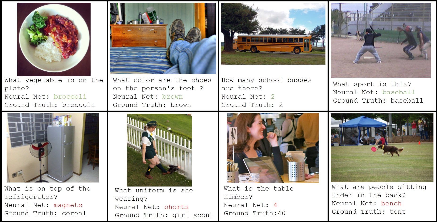
In this blog post, I’ll talk about the Visual Question Answering problem, and I’ll also present neural network based approaches for same. The source code for this blog post is written in Python and Keras, and is available on Github.
An year or so ago, a chatbot named Eugene Goostman made it to the mainstream news, after having been reported as the first computer program to have passed the famed Turing Test in an event organized at the University of Reading. While the organizers hailed it as a historical achievement, most of the scientific community wasn’t impressed. This leads us to the question: Is the Turing Test, in its original form, a suitable test for AI in the modern day?
In the last couple of years, a number of papers (like this paper from JHU/Brown, and this one from MPI) have suggested that the task of Visual Question Answering (VQA, for short) can be used as an alternative Turing Test. The task involves answering an open-ended question (or a series of questions) about an image. An example is shown below:
Image from visualqa.org
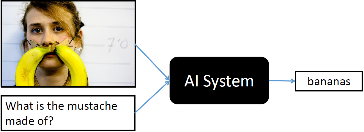
The AI system needs to solve a number of sub-problems in Natural Language Processing and Computer Vision, in addition to being able to perform some kind of “common-sense” reasoning. It needs to localize the subject being referenced (the woman’s face, and more specifically the region around her lips), needs to detect objects (the banana), and should also have some common-sense knowledge that the word mustache is often used to refer to markings or objects on the face that are not actually mustaches (like milk mustaches). Since the problem cuts through two two very different modalities (vision and text), and requires high-level understanding of the scene, it appears to be an ideal candidate for a true Turing Test. The problem also has real world applications, like helping the visually impaired.
A few days ago, the Visual QA Challenge was launched, and along with it came a large dataset (~750K questions on ~250K images). After the MS COCO Image Captioning Challenge sparked a lot of interest in problem of image captioning (or was it the interest that led to the challenge?), the time seems ripe to move onto a much harder problem at the intersection of NLP and Vision.
This post will present ways to model this problem using Neural Networks, exploring both Feedforward Neural Networks, and the much more exciting Recurrent Neural Networks (LSTMs, to be specific). If you do not know much about Neural Networks, then I encourage you to check these two awesome blogs: Colah’s Blog and Karpathy’s Blog. Specifically, check out the posts on Recurrent Neural Nets, Convolutional Neural Nets and LSTM Nets. The models in this post take inspiration from this ICCV 2015 paper, this ICCV 2015 paper, and this NIPS 2015 paper.
Generating Answers
An important aspect of solving this problem is to have a system that can generate new answers. While most of the answers in the VQA dataset are short (1-3 words), we would still like to a have a system that can generate arbitrarily long answers, keeping up with our spirit of the Turing test. We can perhaps take inspiration from papers on Sequence to Sequence Learning using RNNs, that solve a similar problem when generating translations of arbitrary length. Multi-word methods have been presented for VQA too. However, for the purpose of this blog post, we will ignore this aspect of the problem. We will select the 1000 most frequent answers in the VQA training dataset, and solve the problem in a multi-class classification setting. These top 1000 answers cover over 80% of the answers in the VQA training set, so we can still expect to get reasonable results.
The Feedforward Neural Model
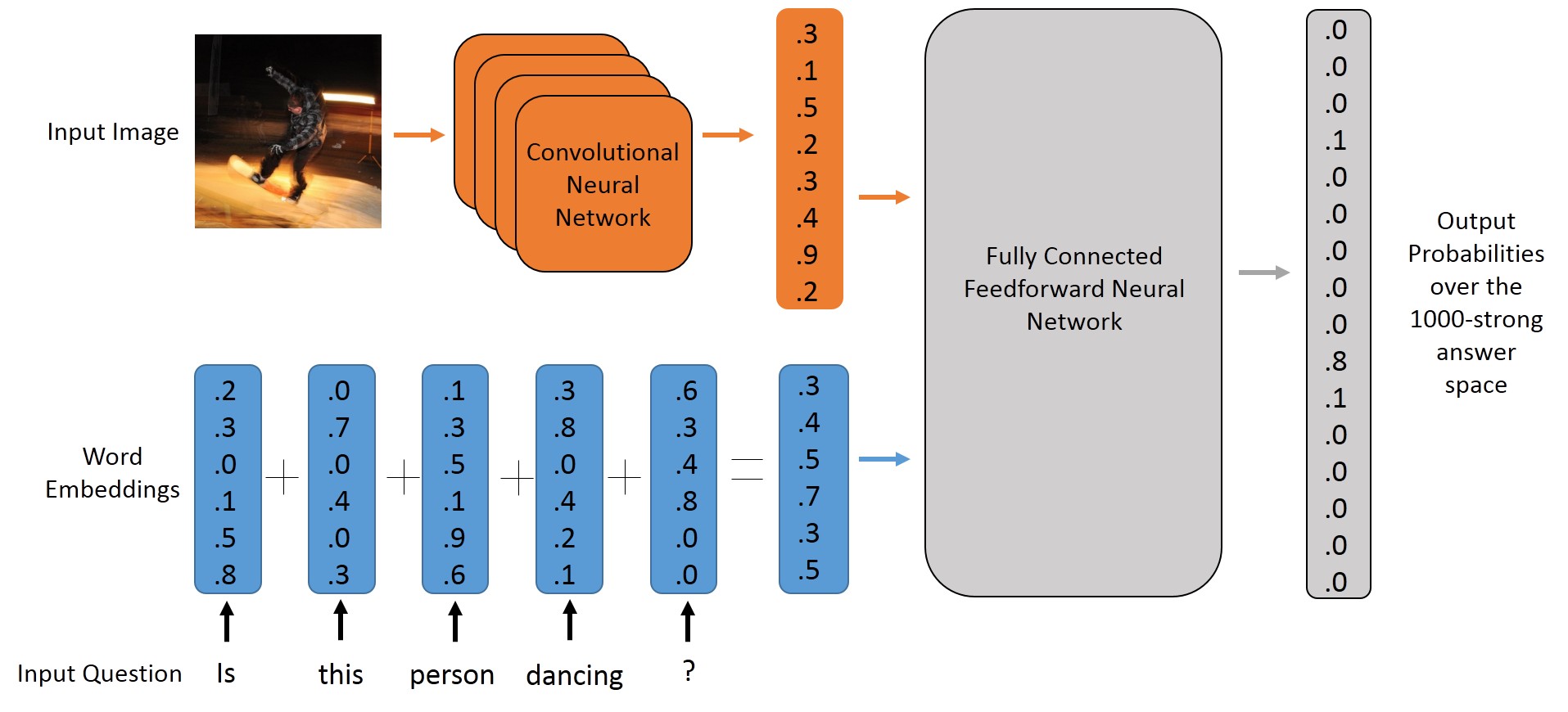
To get started, let’s first try to model the problem using a MultiLayer Perceptron. An MLP is a simple feedforward neural net that maps a feature vector (of fixed length) to an appropriate output. In our problem, this output will be a probability distribution over the set of possible answers. We will be using Keras, an awesome deep learning library based on Theano, and written in Python. Setting up Keras is fairly easy, just have a look at their readme to get started.
In order to use the MLP model, we need to map all our input questions and images to a feature vector of fixed length. We perform the following operations to achieve this:
-
For the question, we transform each word to its word vector, and sum up all the vectors. The length of this feature vector will be same as the length of a single word vector, and the word vectors (also called embeddings) that we use have a length of
300. -
For the image, we pass it through a Deep Convolutional Neural Network (the well-known VGG Architecture), and extract the activation from the second last layer (before the softmax layer, that is). Size of this feature vector is
4096.
Once we have generated the feature vectors, all we need to do now is to define a model in Keras, set up a cost function and an optimizer, and we’re good to go.
The following Keras code defines a multi-layer perceptron with two hidden layers, 1024 hidden units in each layer and dropout layers in the middle for regularization. The final layer is a softmax layer, and is responsible for generating the probability distribution over the set of possible answers. I have used the categorical_crossentropy loss function since it is a multi-class classification problem. The rmsprop method is used for optimzation. You can try experimenting with other optimizers, and see what kind of learning curves you get.
1 | |
Have a look at the entire python script to see the code for generating the features and training the network. It does not access the hard disk once the training begins, and uses about ~4GB of RAM. You can reduce memory usage by lowering the batchSize variable, but that would also lead to longer training times. It is able to process over 215K image-question pairs in less than 160 seconds/epoch when working on a GTX 760 GPU with a batch size of 128. I ran my experiments for 100 epochs.
The Recurrent Neural Model
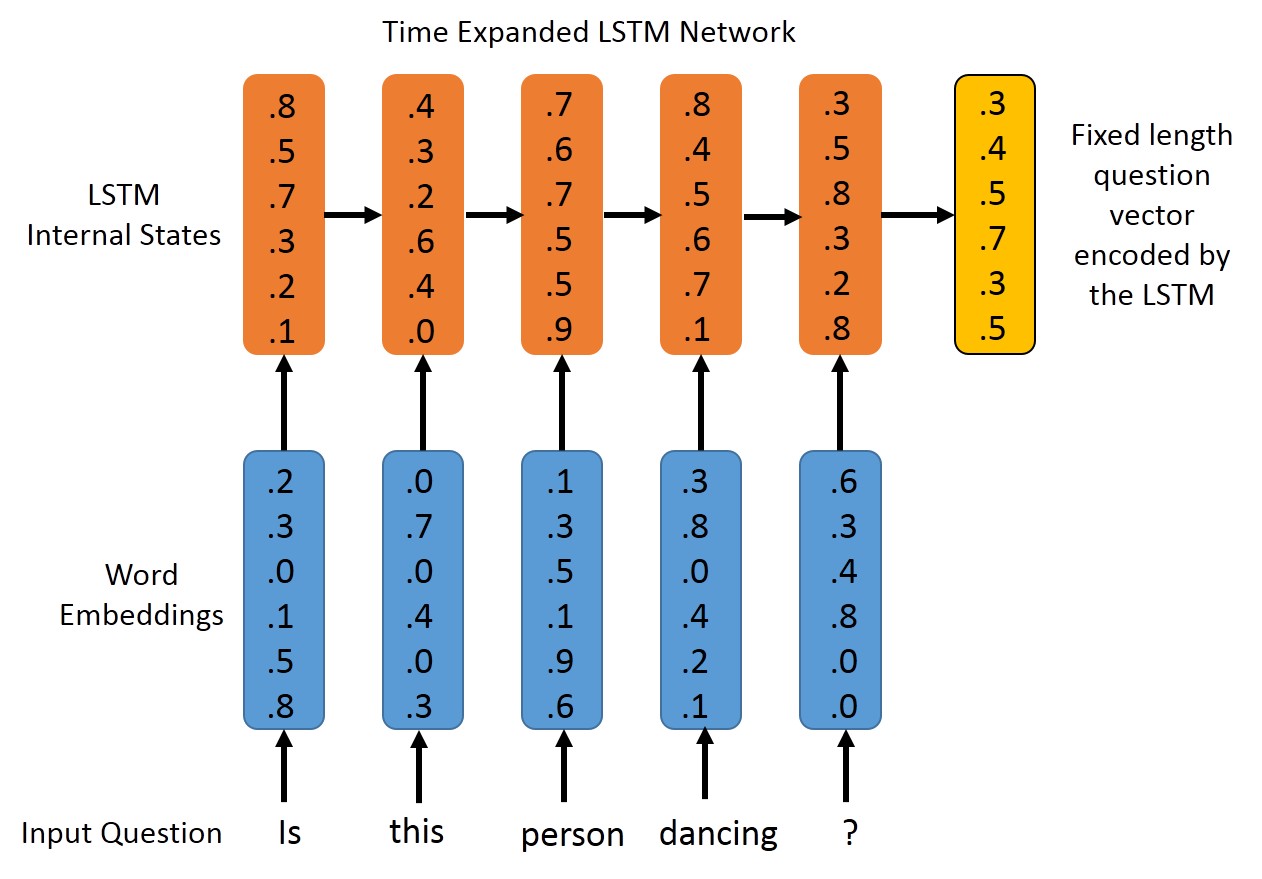
A drawback of the previous approach is that we ignore the sequential nature of the questions. Regardless of what order the words appear in, we’ll get the same vector representing the question, à la bag-of-words (BOW). A way to tackle this limitation is by use of Recurrent Neural Networks, which are well-suited for sequential data. We’ll be using LSTMs here, since they avoid some common nuances of vanilla RNNs, and often give a slightly better performance. You can also experiment with other recurrent layers in Keras, such as GRU. The word vectors corresponding to the tokens in the question are passed to an LSTM in a sequential fashion, and the output of the LSTM (from its output gate) after all the tokens have been passed is chosen as the representation for the entire question. This fixed length vector is concatenated with the 4096 dimensional CNN vector for the image, and passed on to a multi-layer perceptron with fully connected layers. The last layer is once again softmax, and provides us with a probability distribution over the possible outputs.
1 | |
A single train_on_batch method call in Keras expects the sequences to be of the same length (so that is can be represented as a Theano Tensor). There has been a lot of discussion regarding training LSTMs with variable length sequences, and I used the following technique: Sorted all the questions by their length, and then processed them in batches of 128 while training. Most batches had questions of the same length (say 9 or 10 words), and there was no need of zero-padding. For the few batched that did have questions of varying length, the shorter questions were zero-padded. I was able to achieve a training speed of 200 seconds/epoch on a GTX 760 GPU.
Show me the numbers
I trained my system on the Training Set of the VQA dataset, and evaluated performance on the validation set, following the rules of the VQA challenge. The answer produced by the Neural Net is checked against every answer provided by humans (there are ten human answers for every question). If the answer produced by the neural net exactly matches at least three of the ten answers, then we classify it as a correct prediction. Here is the performance of the models that I trained:
| Model | Accuracy |
|---|---|
| BOW+CNN | 48.46% |
| LSTM-Language only | 44.17% |
| LSTM+CNN | 51.63% |
Update: The results that I reported earlier were based on a metric slightly different from the ones used on VQA. They have since been updated. Also, I was able to obtain a performance of 53.34% on the test-dev set (LSTM+CNN), which is practically the same as those set by the VQA authors in their LSTM baseline.
It’s interesting to see that even a “blind” model is able to obtain an accuracy of 44.17%. This shows that the model is pretty good at guessing the answers once it has identified the type of question. The LSTM+CNN model shows an improvement of about 3% as compared to the Feedforward Model (BOW+CNN), which tells us that the temporal structure of the question is indeed helpful. These results are in line with what was obtained in the original VQA paper. However, the results reported in the paper were on the test set (trained on train+val), while we have evaluated on the validation set (trained on only train). If we learn a model on both the training and the validation data, then we can expect a significant improvement in performance since the number of training examples will increase by 50%. Finally, there is a lot of scope for hyperparameter tuning (number of hidden units, number of MLP hidden layers, number of LSTM layers, dropout or no dropout etc.).
I carried out my experiments for 100 epochs, and observed the following curve:
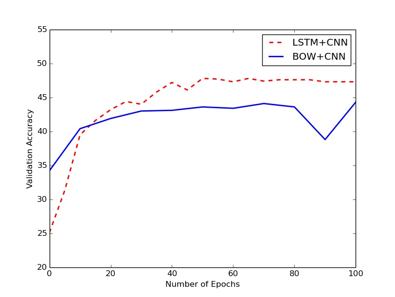
The LSTM+CNN model flattens out in performance after about 50 epochs. The BOW+CNN also showed similar behavior, but took a surprising dive at epoch 90, which was soon rectified by the 100th epoch. I’ll probably re-initialize and run the models for 500 epochs, and see if such behavior is seen again or not. Update: I did run it once more, and the dip was not observed!
A note on word embeddings
We have a number of choices when using word embeddings, and I experimented with three of them:
GloVe Word Embeddings trained on the common-crawl: These gave the best performance, and all results reported here are using these embeddings.
Goldberg and Levy 2014: These are the default embeddings that come with spaCy, and they gave significantly worse results.
Embeddings Trained on the VQA questions: I used Gensim’s word2vec implementation to train my own embeddings on the questions in the training set of the VQA dataset. The performance was similar to, but slighly worse than the GloVe embeddings. This is primarily because the VQA training set alone is not sufficiently large (~2.5m words) to get reasonable word vectors, especially for less common words.