By the time I’d finished building the model in my last blog, I’d started to overload my computer’s RAM and CPU, so much so that I couldn’t add any more features. One solution could be for me to upgrade my hardware, or rent out a cluster in the cloud, but I’m trying to save money at the moment. So today I’m going to restructure my predictive solution into separate predictive models, each of which do not individually overload my computer, but which are combined via stacking to give an overall solution that is more predictive than any of the individual models.

Stacking would also allow us to answer Bobby’s question:
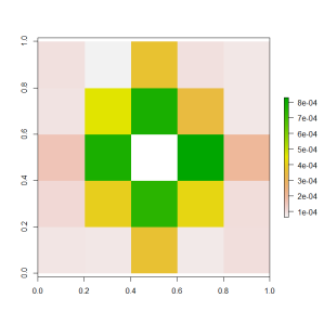
I thought it was interesting how the importance chart didn’t show any one individual pixel as being significant. Is there another similar importance chart or metric that can show the importance of a combination of pixels?
So let’s start by breaking up the current monolithic model into discrete chunks. Once we have done this, it will be easier for us to add new features (which I will do in the next blog). I will store the predicted outputs from each model in image format with separate folders for each model.

The R script for creating the individual models is primarily recycled from my past blogs. Since images contain integer values for pixel brightness, one may argue that storing the predicted values as images loses some of the information content, but the rounding of floating point values to integer values only affects the precision by a maximum of 0.2%, and the noise in the predicted values is an order of magnitude greater than that. If you want that fractional extra predictive power, then I leave it to you to adapt the script to write the floating point predictions into a data.table.
The linear transformation model was developed here, and just involves a linear transformation, then constraining the output to be in the [0, 1] range.

The thresholding model was developed here, and involves a combination of adaptive thresholding processes, each with different sizes of localisation ranges, plus a global thresholding process. But this time we will use xgboost instead of gbm.

The edge model was developed here, and involves a combination of canny edge detection and image morphology.

The background removal model was developed here, and involves the use of median filters. An xgboost model is used to combine the median filter results.

The spacial model was developed here, and involves the use of a sliding window and xgboost.
There are many ways that the predictions of the models could be ensembled together. I have used an xgboost model because I want to allow for the complexity of the problem that is being solved.
 The graph above answers Bobby’s question – when considered together, the nearby pixels provide most of the additional predictive power beyond that of the raw pixel brightness. It seems that the key to separating dark text from noise is to consider how the pixel fits into the local region within the image.Now that we have set up a stacking model structure, we can recommence the process of adding more image processing and features to the model. And that’s what the next blog will do…
Like this:
Like Loading…
Related