In today’s tutorial, we are going to discuss the Keras Conv2D class, including the most important parameters you need to tune when training your own Convolutional Neural Networks (CNNs). From there we are going to use the Keras Conv2D class to implement a simple CNN. We’ll then train and evaluate this CNN on the CALTECH-101 dataset.
The inspiration for today’s post came from PyImageSearch reader, Danny.
Danny asked:
Hi Adrian, I’m having some trouble understanding the parameters to Keras’ Conv2D class. Which ones are the important ones? Which ones should I just leave at their default values? I’m a bit new to deep learning so I’m a bit confused on how to choose the parameter values when creating my own CNN.
Danny asks a great question — there are quite a few parameters to Keras’ Conv2D class. The sheer number can be a bit overwhelming if you’re new to the world of computer vision and deep learning.
In today’s tutorial I’m going to discuss each of the parameters to the Keras Conv2D class, explain each one, and provide examples of situations where and when you would want to set specific values, enabling you to:
-
Quickly determine if you need to utilize a specific parameter to the Keras Conv2D class
-
Decide on a proper valuefor that specific parameter
-
Effectively train your own Convolutional Neural Network
Overall, my goal is to help reduce any confusion, anxiety, or frustration when using Keras’ Conv2D class. After going through this tutorial you will have a strong understanding of the Keras Conv2D parameters.
To learn more about the Keras Conv2D class and convolutional layers, just keep reading!
Keras Conv2D and Convolutional Layers
In the first part of this tutorial, we are going to discuss the parameters to the Keras Conv2D class.
From there we are going to utilize the Conv2D class to implement a simple Convolutional Neural Network.
We’ll then take our CNN implementation and then train it on the CALTECH-101 dataset.
Finally, we’ll evaluate the network and examine its performance.
Let’s go ahead and get started!
The Keras Conv2D class
The Keras Conv2D class constructor has the following signature:
| keras.layers.Conv2D(filters, kernel_size, strides=(1, 1), padding=’valid’, data_format=None, dilation_rate=(1, 1), activation=None, use_bias=True, kernel_initializer=’glorot_uniform’, bias_initializer=’zeros’, kernel_regularizer=None, bias_regularizer=None, activity_regularizer=None, kernel_constraint=None, bias_constraint=None) |
padding=’valid’, data_format=None, dilation_rate=(1, 1),
bias_initializer=’zeros’, kernel_regularizer=None,
kernel_constraint=None, bias_constraint=None)
Looks a bit overwhelming, right?
How in the world are you supposed to properly set these values?
No worries — let’s examine each of these parameters individually, giving you a strong understanding of not only what each parameter controls but also how to properly set each parameter as well.
filters
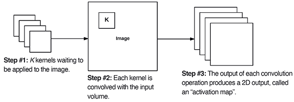
Figure 1: The Keras Conv2D parameter, filters determines the number of kernels to convolve with the input volume. Each of these operations produces a 2D activation map.
The first required Conv2D parameter is the number of filters that the convolutional layer will learn.
Layers early in the network architecture (i.e., closer to the actual input image) learn fewer convolutional filters while layers deeper in the network (i.e., closer to the output predictions) will learn more filters.
Conv2D layers in between will learn more filters than the early Conv2D layers but fewer filters than the layers closer to the output. Let’s go ahead and take a look at an example:
| model.add(Conv2D(32, (3, 3), padding=”same”, activation=”relu”))model.add(MaxPooling2D(pool_size=(2, 2)))…model.add(Conv2D(64, (3, 3), padding=”same”, activation=”relu”))model.add(MaxPooling2D(pool_size=(2, 2)))…model.add(Conv2D(128, (3, 3), padding=”same”, activation=”relu”))model.add(MaxPooling2D(pool_size=(2, 2)))…model.add(Activation(“softmax”)) |
model.add(MaxPooling2D(pool_size=(2, 2)))
model.add(Conv2D(64, (3, 3), padding=”same”, activation=”relu”))
…
model.add(MaxPooling2D(pool_size=(2, 2)))
model.add(Activation(“softmax”))
On Line 1 we learn a total of 32 filters. Max pooling is then used to reduce the spatial dimensions of the output volume.
We then learn 64 filters on Line 4. Again max pooling is used to reduce the spatial dimensions.
The final Conv2D layer learns 128 filters.
Notice at as our output spatial volume is decreasing our number of filters learned is increasing — this is a common practice in designing CNN architectures and one I recommend you do as well. As far as choosing the appropriate number of filters , I nearly always recommend using powers of 2 as the values.
You may need to tune the exact value depending on (1) the complexity of your dataset and (2) the depth of your neural network, but I recommend starting with filters in the range [32, 64, 128] in the earlier and increasing up to [256, 512, 1024] in the deeper layers.
Again, the exact range of the values may be different for you, but start with a smaller number of filters and only increase when necessary.
kernel_size
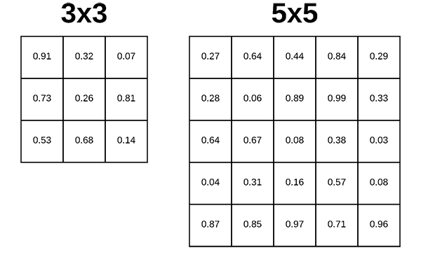
Figure 2: The Keras deep learning Conv2D parameter, filter_size, determines the dimensions of the kernel. Common dimensions include 1×1, 3×3, 5×5, and 7×7 which can be passed as (1, 1), (3, 3), (5, 5), or (7, 7) tuples.
The second required parameter you need to provide to the Keras Conv2D class is the kernel_size , a 2-tuple specifying the width and height of the 2D convolution window.
The kernel_size must be an odd integer as well.
Typical values for kernel_size include: (1, 1) , (3, 3) , (5, 5) , (7, 7) . It’s rare to see kernel sizes larger than 7×7.
So, when do you use each?
If your input images are greater than 128×128 you may choose to use a kernel size > 3 to help (1) learn larger spatial filters and (2) to help reduce volume size.
Other networks, such as VGGNet, exclusively use (3, 3) filters throughout the entire network.
More advanced architectures such as Inception, ResNet, and SqueezeNet design entire micro-architectures which are “modules” inside the network that learn local features at different scales (i.e., 1×1, 3×3, and 5×5) and then combine the outputs.
A great example can be seen in the Inception module below:
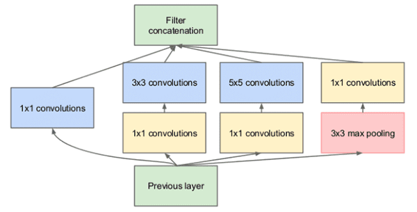
Figure 3: The Inception/GoogLeNet CNN architecture uses “micro-architecture” modules inside the network that learn local features at different scales (filter_size) and then combine the outputs.
The Residual module in the ResNet architecture uses 1×1 and 3×3 filters as a form of dimensionality reduction which helps to keep the number of parameters in the network low (or as low as possible given the depth of the network):
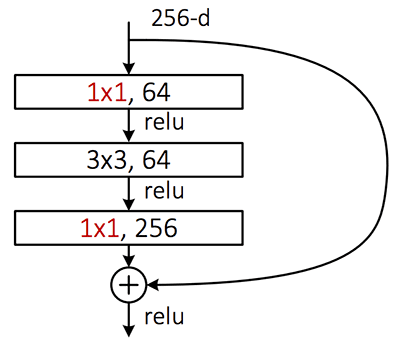
Figure 4: The ResNet “Residual module” uses 1×1 and 3×3 filters for dimensionality reduction. This helps keep the overall network smaller with fewer parameters.
So, how should you choose your filter_size ?
First, examine your input image — is it larger than 128×128?
If so, consider using a 5×5 or 7×7 kernel to learn larger features and then quickly reduce spatial dimensions — then start working with 3×3 kernels:
| model.add(Conv2D(32, (7, 7), activation=”relu”))…model.add(Conv2D(32, (3, 3), activation=”relu”)) |
…
If your images are smaller than 128×128 you may want to consider sticking with strictly 1×1 and 3×3 filters.
And if you intend on using ResNet or Inception-like modules you’ll want to implement the associated modules and architectures by hand. Covering how to implement these modules is outside the scope of this tutorial, but if you’re interested in learning more about them (including how to hand-code them), please refer to my book, Deep Learning for Computer Vision with Python.
strides
The strides parameter is a 2-tuple of integers, specifying the “step” of the convolution along the x and y axis of the input volume.
The strides value defaults to (1, 1) , implying that:
-
A given convolutional filter is applied to the current location of the input volume
-
The filter takes a 1-pixel step to the right and again the filter is applied to the input volume
-
This process is performed until we reach the far-right border of the volume in which we move our filter one pixel down and then start again from the far left
Typically you’ll leave the strides parameter with the default (1, 1) value; however, you may occasionally increase it to (2, 2) to help reduce the size of the output volume (since the step size of the filter is larger).
Typically you’ll see strides of 2×2 as a replacement to max pooling:
| model.add(Conv2D(128, (3, 3), strides=(1, 1), activation=”relu”))model.add(Conv2D(128, (3, 3), strides=(1, 1), activation=”relu”))model.add(Conv2D(128, (3, 3), strides=(2, 2), activation=”relu”)) |
model.add(Conv2D(128, (3, 3), strides=(1, 1), activation=”relu”))
Here we can see our first two Conv2D layers have a stride of 1×1. The final Conv2D layer; however, takes the place of a max pooling layer, and instead reduces the spatial dimensions of the output volume via strided convolution.
In 2014, Springenber et al. published a paper entitled Striving for Simplicity: The All Convolutional Net which demonstrated that replacing pooling layers with strided convolutions can increase accuracy in some situations.
ResNet, a popular CNN, has embraced this finding — if you ever look at the source code to a ResNet implementation (or implement it yourself), you’ll see that ResNet replies on strided convolution rather than max pooling to reduce spatial dimensions in between residual modules.
padding

Figure 5: A 3×3 kernel applied to an image with padding. The Keras Conv2D padding parameter accepts either "valid" (no padding) or "same" (padding + preserving spatial dimensions). This animation was contributed to StackOverflow (source).
The padding parameter to the Keras Conv2D class can take on one of two values: valid or same .
With the valid parameter the input volume is not zero-padded and the spatial dimensions are allowed to reduce via the natural application of convolution.
The following example would naturally reduce the spatial dimensions of our volume:
| model.add(Conv2D(32, (3, 3), padding=”valid”)) |
Note: See this tutorial on the basics of convolution if you need help understanding how and why spatial dimensions naturally reduce when applying convolutions.
If you instead want to preserve the spatial dimensions of the volume such that the output volume size matches the input volume size, then you would want to supply a value of same for the padding :
| model.add(Conv2D(32, (3, 3), padding=”same”)) |
While the default Keras Conv2D value is valid I will typically set it to same for the majority of the layers in my network and then either reduce spatial dimensions of my volume by either:
-
Max pooling
-
Strided convolution
I would recommend that you use a similar approach to padding with the Keras Conv2D class as well.
data_format
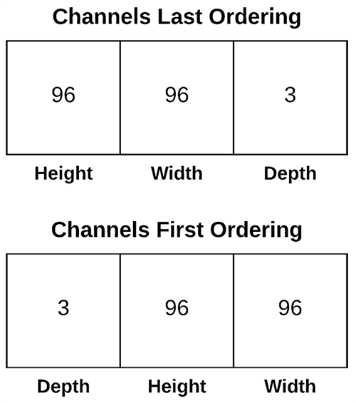
Figure 6: Keras, as a high-level framework, supports multiple deep learning backends. Thus, it includes support for both “channels last” and “channels first” channel ordering.
The data format value in the Conv2D class can be either channels_last or channels_first :
-
The TensorFlow backend to Keras uses channels last ordering.
-
The Theano backend uses channels first ordering.
You typically shouldn’t have to ever touch this value as Keras for two reasons:
- You are more than likely using the TensorFlow backend to Keras
And if not, you’ve likely already updated your ~/.keras/keras.json configuration file to set your backend and associated channel ordering
My advice is to never explicitly set the data_format in your Conv2D class unless you have a very good reason to do so.
dilation_rate
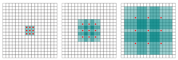
Figure 7: The Keras deep learning Conv2D parameter, dilation_rate, accepts a 2-tuple of integers to control dilated convolution (source).
The dilation_rate parameter of the Conv2D class is a 2-tuple of integers, controlling the dilation rate for dilated convolution. Dilated convolution is a basic convolution only applied to the input volume with defined gaps, as Figure 7 above demonstrates.
You may use dilated convolution when:
-
You are working with higher resolution images but fine-grained details are still important
-
You are constructing a network with fewer parameters
Discussing dilated convolution is outside the scope of this tutorial so if you are interested in learning more, please refer to this tutorial.
activation
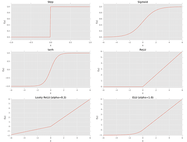
Figure 8: Keras provides a number of common activation functions. The activation parameter to Conv2D is a matter of convenience and allows the activation function for use after convolution to be specified.
The activation parameter to the Conv2D class is simply a convenience parameter, allowing you to supply a string specifying the name of the activation function you want to apply after performing the convolution.
In the following example we perform convolution and then apply a ReLU activation function:
| model.add(Conv2D(32, (3, 3), activation=”relu”)) |
The above code is equivalent to:
| model.add(Conv2D(32, (3, 3)))model.add(Activation(“relu”)) |
model.add(Activation(“relu”))
My advice?
Use the activation parameter if you and if it helps keep your code cleaner — it’s entirely up to you and won’t have an impact on the performance of your Convolutional Neural Network.
use_bias
The use_bias parameter of the Conv2D class controls whether a bias vector is added to the convolutional layer.
Typically you’ll want to leave this value as True , although some implementations of ResNet will leave the bias parameter out.
I recommend keep the bias unless you have a good reason not to.
kernel_initializer and bias_initializer
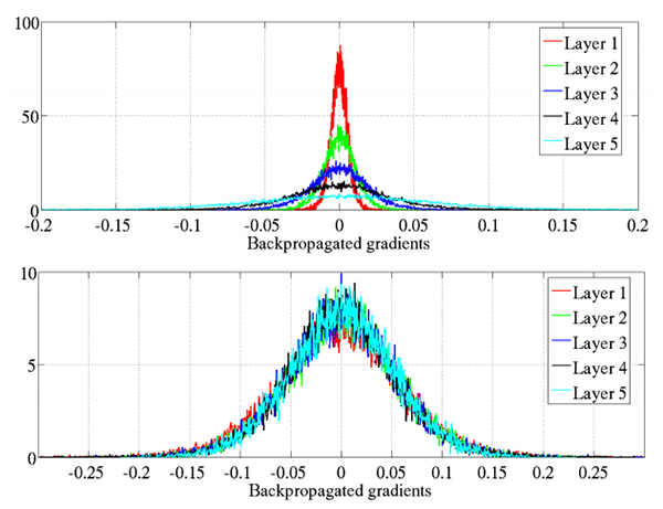
Figure 9: Keras offers a number of initializers for the Conv2D class. Initializers can be used to help train deeper neural networks more effectively.
The kernel_initializer controls the initialization method used to initialize all values in the Conv2D class prior to actually training the network.
Similarly, the bias_initializer controls how the bias vector is initialized before training starts.
A full list of initializers can be found in the Keras documentation; however, here is what I recommend:
Leave the bias_initialization alone — it will by default filled with zeros (you’ll rarely if ever, have to change the bias initialization method. The kernel_initializer defaults to glorot_uniform , the Xavier Glorot uniform initialization method, which is perfectly fine for the majority of tasks; however, for deeper neural networks you may want to use he_normal (MSRA/He et al. initialization) which works especially well when your network has a large number of parameters (i.e., VGGNet).
In the vast majority of CNNs I implement I am either using glorot_uniform or he_normal — I recommend you do the same unless you have a specific reason to use a different initializer.
kernel_regularizer, bias_regularizer, and activity_regularizer
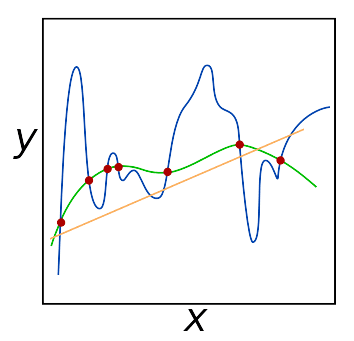
Figure 10: Regularization hyperparameters should be adjusted especially when working with large datasets and really deep networks. The kernel_regularizer parameter in particular is one that I adjust often to reduce overfitting and increase the ability for a model to generalize to unfamiliar images.
The kernel_regularizer , bias_regularizer , and activity_regularizer control the type and amount of regularization method applied to the Conv2D layer.
Applying regularization helps you to:
-
Reduce the effects of overfitting
-
Increase the ability of your model to generalize
When working with large datasets and deep neural networks applying regularization is typically a must.
Normally you’ll encounter either L1 or L2 regularization being applied — I will use L2 regularization on my networks if I detect signs of overfitting:
| from keras.regularizers import l2…model.add(Conv2D(32, (3, 3), activation=”relu”), kernel_regularizer=l2(0.0005)) |
…
kernel_regularizer=l2(0.0005))
The amount of regularization you apply is a hyperparameter you will need to tune for your own dataset, but I find values of 0.0001-0.001 are good ranges to start with.
I would suggest leaving your bias regularizer alone — regularizing the bias typically has very little impact on reducing overfitting.
I also suggest leaving the activity_regularizer at its default value (i.e., no activity regularization).
While weight regularization methods operate on weights themselves, f(W), where f is the activation function and W are the weights, an activity regularizer instead operates on the outputs, f(O), where O is the outputs of a layer.
Unless there is a very specific reason you’re looking to regularize the output it’s best to leave this parameter alone.
kernel_constraint and bias_constraint
The final two parameters to the Keras Conv2D class are the kernel_constraint and bias_constraint .
These parameters allow you to impose constraints on the Conv2D layer, including non-negativity, unit normalization, and min-max normalization.
You can see the full list of supported constraints in the Keras documentation.
Again, I would recommend leaving both the kernel constraint and bias constraint alone unless you have a specific reason to impose constraints on the Conv2D layer.
The CALTECH-101 (subset) dataset
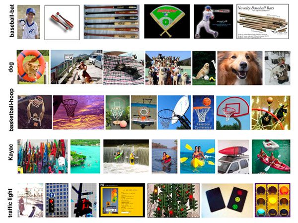
Figure 11: The CALTECH-101 dataset consists of 101 object categories with 40-80 images per class. The dataset for today’s blog post example consists of just 4 of those classes: faces, leopards, motorbikes, and airplanes (source).
The CALTECH-101 dataset is a dataset of 101 object categories with 40 to 800 images per class.
Most images have approximately 50 images per class.
The goal of the dataset is to train a model capable of predicting the target class.
Prior to the resurgence of neural networks and deep learning, the state-of-the-art accuracy on was only ~65%.
However, by using Convolutional Neural Networks, it’s been possible to achieve 90%+ accuracy (as He et al. demonstrated in their 2014 paper, Spatial Pyramid Pooling in Deep Convolutional Networks for Visual Recognition).
Today we are going to implement a simple yet effective CNN that is capable of achieving 96%+ accuracy, on a 4-class subset of the dataset:
-
Faces: 436 images
-
Leopards: 201 images
-
Motorbikes: 799 images
-
Airplanes: 801 images
The reason we are using a subset of the dataset is so you can easily follow along with this example and train the network from scratch, even if you do not have a GPU.
Again, the purpose of this tutorial is not meant to deliver state-of-the-art results on CALTECH-101 — it’s instead meant to teach you the fundamentals of how to use Keras’ Conv2D class to implement and train a custom Convolutional Neural Network.
Downloading the dataset and source code
Interested in following along with today’s tutorial? If so, you’ll need to download both:
-
The source code to this post (using the “Downloads”section of the post)
-
The CALTECH-101 dataset
To download the source code to this post you can use this link. Adrian: Please add link
After you have downloaded the .zip of the source code, unarchive it, and then change directory into the keras-conv2d-example directory:
| $ cd /path/to/keras-conv2d-example |
From there, use the following wget command to download and unarchive the CALTECH-101 dataset:
| $ wget http://www.vision.caltech.edu/Image_Datasets/Caltech101/101_ObjectCategories.tar.gz$ tar -zxvf 101_ObjectCategories.tar.gz |
$ tar -zxvf 101_ObjectCategories.tar.gz
Now that we’ve downloaded our code and dataset we can move on inspecting the project structure.
Project structure
To see how our project is organized, simply use the tree command:
| 12345678910111213141516171819 | $ tree –dirsfirst -L 2 -v.├── 101_ObjectCategories…│ ├── Faces [436 entries]…│ ├── Leopards [201 entries]│ ├── Motorbikes [799 entries]…│ ├── airplanes [801 entries]…├── pyimagesearch│ ├── init.py│ └── stridednet.py├── 101_ObjectCategories.tar.gz├── train.py└── plot.png 104 directories, 5 files |
2
4
6
8
10
12
14
16
18
.
…
│ ├── Motorbikes [799 entries]
│ ├── airplanes [801 entries]
├── pyimagesearch
│ └── stridednet.py
├── train.py
The first directory, 101_ObjectCategories/ is our dataset that we extracted in the last section. It contains 102 folders, so I eliminated the lines that we don’t care about for today’s blog post. What remains is the subset of four object categories previously discussed.
The pyimagesearch/ module is not pip installable. You must use the “Downloads” to grab the files. Inside the module, you’ll find stridendet.py which contains the StridedNet class.
In addition to stridednet.py , we’ll review train.py in the root folder. Our training script will make use of StridedNet and our small dataset to train a model for example purposes.
The training script will produce a training history plot, plot.png .
A Keras Conv2D Example
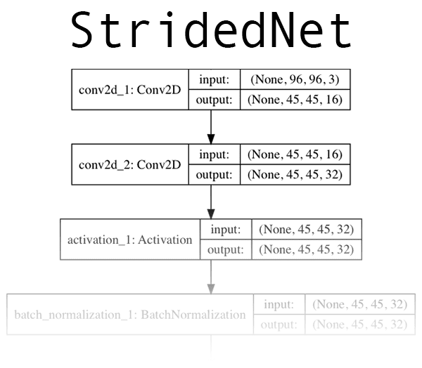
Figure 12: A deep learning CNN dubbed “StridedNet” serves as the example for today’s blog post about Keras Conv2D parameters. Click to expand.
Now that we’re reviewed both (1) how the Keras Conv2D class works and (2) the dataset we’ll be training our network on, let’s go ahead and implement the Convolutional Neural Neural network we’ll be training.
The CNN we’ll be using today, “StridedNet”, is one I made up for the purposes of this tutorial.
StridedNet has three important characteristics:
-
It uses strided convolutions rather than pooling operations to reduce volume size
-
The first CONV layer uses 7×7 filters but all other layers in the network use 3×3 filters (similar to VGG)
-
The MSRA/He et al. normal distribution algorithm is used to initialize all weights in the network
Let’s go ahead and implemented StridedNet now.
Open up a new file, name it stridednet.py , and insert the following code:
| 123456789101112131415161718192021222324 | # import the necessary packagesfrom keras.models import Sequentialfrom keras.layers.normalization import BatchNormalizationfrom keras.layers.convolutional import Conv2Dfrom keras.layers.core import Activationfrom keras.layers.core import Flattenfrom keras.layers.core import Dropoutfrom keras.layers.core import Densefrom keras import backend as K class StridedNet: @staticmethod def build(width, height, depth, classes, reg, init=”he_normal”): # initialize the model along with the input shape to be # “channels last” and the channels dimension itself model = Sequential() inputShape = (height, width, depth) chanDim = -1 # if we are using “channels first”, update the input shape # and channels dimension if K.image_data_format() == “channels_first”: inputShape = (depth, height, width) chanDim = 1 |
2
4
6
8
10
12
14
16
18
20
22
24
from keras.models import Sequential
from keras.layers.convolutional import Conv2D
from keras.layers.core import Flatten
from keras.layers.core import Dense
@staticmethod
# initialize the model along with the input shape to be
model = Sequential()
chanDim = -1
# if we are using “channels first”, update the input shape
if K.image_data_format() == “channels_first”:
chanDim = 1
All of our Keras modules are imported on Lines 2-9, namely Conv2D .
Our StridedNet class is defined on Line 11 with a single build method on Line 13.
The build method accepts six parameters:
width : Image width in pixels.
height : The image height in pixels.
depth : The number of channels for the image.
classes : The number of classes the model needs to predict.
reg : Regularization method.
init : The kernel initializer.
The width , height , and depth parameters affect the input volume shape.
For “channels_last” ordering, the input shape is specified on Line 17 where the depth is last.
We can use the Keras backend to check the image_data_format to see if we need to accommodate “channels_first” ordering (Lines 22-24).
Let’s take a lot at how we can build the first three CONV layers:
| 262728293031323334353637383940414243 | # our first CONV layer will learn a total of 16 filters, each # Of which are 7x7 – we’ll then apply 2x2 strides to reduce # the spatial dimensions of the volume model.add(Conv2D(16, (7, 7), strides=(2, 2), padding=”valid”, kernel_initializer=init, kernel_regularizer=reg, input_shape=inputShape)) # here we stack two CONV layers on top of each other where # each layerswill learn a total of 32 (3x3) filters model.add(Conv2D(32, (3, 3), padding=”same”, kernel_initializer=init, kernel_regularizer=reg)) model.add(Activation(“relu”)) model.add(BatchNormalization(axis=chanDim)) model.add(Conv2D(32, (3, 3), strides=(2, 2), padding=”same”, kernel_initializer=init, kernel_regularizer=reg)) model.add(Activation(“relu”)) model.add(BatchNormalization(axis=chanDim)) model.add(Dropout(0.25)) |
27
29
31
33
35
37
39
41
43
# Of which are 7x7 – we’ll then apply 2x2 strides to reduce
model.add(Conv2D(16, (7, 7), strides=(2, 2), padding=”valid”,
input_shape=inputShape))
# here we stack two CONV layers on top of each other where
model.add(Conv2D(32, (3, 3), padding=”same”,
model.add(Activation(“relu”))
model.add(Conv2D(32, (3, 3), strides=(2, 2), padding=”same”,
model.add(Activation(“relu”))
model.add(Dropout(0.25))
Each Conv2D is stacked on the network with model.add .
Notice that for the first Conv2D layer, we’ve explicitly specified our inputShape so that the CNN architecture has somewhere to start and build off of. Then, from here forward, each time model.add is called, the previous layer acts as the input to the next layer.
Taking into account the parameters to Conv2D discussed previously, you’ll notice that we are using strided convolution to reduce spatial dimensions rather than pooling operations.
ReLU activation is applied (refer to Figure 8) along with batch normalization and dropout.
I nearly always recommend batch normalization because it tends to stabilize training and make tuning hyperparameters easier. That said, it can double or triple your training time. Use it wisely.
Dropout’s purpose is to help your network generalize and not overfit. Neurons from the current layer, with probability p, will randomly disconnect from neurons in the next layer so that the network has to rely on the existing connections. I highly recommend utilizing dropout.
Let’s take a look at more layers of StridedNet:
| 45464748495051525354555657585960616263646566 | # stack two more CONV layers, keeping the size of each filter # as 3x3 but increasing to 64 total learned filters model.add(Conv2D(64, (3, 3), padding=”same”, kernel_initializer=init, kernel_regularizer=reg)) model.add(Activation(“relu”)) model.add(BatchNormalization(axis=chanDim)) model.add(Conv2D(64, (3, 3), strides=(2, 2), padding=”same”, kernel_initializer=init, kernel_regularizer=reg)) model.add(Activation(“relu”)) model.add(BatchNormalization(axis=chanDim)) model.add(Dropout(0.25)) # increase the number of filters again, this time to 128 model.add(Conv2D(128, (3, 3), padding=”same”, kernel_initializer=init, kernel_regularizer=reg)) model.add(Activation(“relu”)) model.add(BatchNormalization(axis=chanDim)) model.add(Conv2D(128, (3, 3), strides=(2, 2), padding=”same”, kernel_initializer=init, kernel_regularizer=reg)) model.add(Activation(“relu”)) model.add(BatchNormalization(axis=chanDim)) model.add(Dropout(0.25)) |
46
48
50
52
54
56
58
60
62
64
66
# as 3x3 but increasing to 64 total learned filters
kernel_initializer=init, kernel_regularizer=reg))
model.add(BatchNormalization(axis=chanDim))
kernel_initializer=init, kernel_regularizer=reg))
model.add(BatchNormalization(axis=chanDim))
model.add(Conv2D(128, (3, 3), padding=”same”,
model.add(Activation(“relu”))
model.add(Conv2D(128, (3, 3), strides=(2, 2), padding=”same”,
model.add(Activation(“relu”))
model.add(Dropout(0.25))
The deeper the network goes, the more filters we learn.
At the end of most networks we add a fully connected layer:
| 68697071727374757677787980 | # fully-connected layer model.add(Flatten()) model.add(Dense(512, kernel_initializer=init)) model.add(Activation(“relu”)) model.add(BatchNormalization()) model.add(Dropout(0.5)) # softmax classifier model.add(Dense(classes)) model.add(Activation(“softmax”)) # return the constructed network architecture return model |
69
71
73
75
77
79
model.add(Flatten())
model.add(Activation(“relu”))
model.add(Dropout(0.5))
# softmax classifier
model.add(Activation(“softmax”))
# return the constructed network architecture
A single fully connected layer with 512 nodes is appended to the CNN.
Finally, a “softmax” classifier is added to the network — the output of this layer are the prediction values themselves.
That’s a wrap.
As you can see, Keras syntax is quite straightforward once you know what the parameters mean ( Conv2D having the potential for quite a few parameters).
Let’s learn how to write a script to train StridedNet with some data!
Implementing the training script
Now that we have implemented our CNN architecture, let’s create the driver script used to train the network.
Open up the train.py file an insert the following code:
| 123456789101112131415161718 | # set the matplotlib backend so figures can be saved in the backgroundimport matplotlibmatplotlib.use(“Agg”) # import the necessary packagesfrom pyimagesearch.stridednet import StridedNetfrom sklearn.preprocessing import LabelBinarizerfrom sklearn.model_selection import train_test_splitfrom sklearn.metrics import classification_reportfrom keras.preprocessing.image import ImageDataGeneratorfrom keras.optimizers import Adamfrom keras.regularizers import l2from imutils import pathsimport matplotlib.pyplot as pltimport numpy as npimport argparseimport cv2import os |
2
4
6
8
10
12
14
16
18
import matplotlib
from pyimagesearch.stridednet import StridedNet
from sklearn.model_selection import train_test_split
from keras.preprocessing.image import ImageDataGenerator
from keras.regularizers import l2
import matplotlib.pyplot as plt
import argparse
import os
We import our modules and packages on Lines 2-18. Notice that we aren’t importing Conv2D anywhere. Our CNN implementation is contained within stridednet.py and our StridedNet import handles it (Line 6).
Our matplotlib backend is set on Line 3 — this is necessary so we can save our plot as an image file rather than viewing it in the GUI.
We import functionality from sklearn on Lines 7-9:
LabelBinarizer : For “one-hot” encoding our class labels.
train_test_split : For splitting our data such that we have training and evaluation sets.
classification_report : We’ll use this to print statistics from evaluation.
From keras we’ll be using:
ImageDataGenerator : For data augmentation. See last week’s blog post for more information on Keras data generators.
Adam : An optimizer alternative to SGD.
l2 : The regularizer we’ll be using. Scroll up to read about regularizers. Applying regularization reduces overfitting and helps with generalization.
My imutils paths module will be used to grab the paths to our images in the dataset.
We’ll use argparse to handle command line arguments at runtime, and OpenCV ( cv2 ) will be used to load and preprocess images from the dataset.
Let’s go ahead and parse the command line arguments now:
| # construct the argument parser and parse the argumentsap = argparse.ArgumentParser()ap.add_argument(“-d”, “–dataset”, required=True, help=”path to input dataset”)ap.add_argument(“-e”, “–epochs”, type=int, default=50, help=”# of epochs to train our network for”)ap.add_argument(“-p”, “–plot”, type=str, default=”plot.png”, help=”path to output loss/accuracy plot”)args = vars(ap.parse_args()) |
ap = argparse.ArgumentParser()
help=”path to input dataset”)
help=”# of epochs to train our network for”)
help=”path to output loss/accuracy plot”)
Our script can accept three command line arguments:
–dataset : The path to the input dataset.
–epochs : The number of epochs to train for. By default , we’ll train for 50 epochs.
–plot : Our loss/accuracy plot will be output to disk. This argument contains the file path. By default, it is simply “plot.png” .
Let’s prepare to load our dataset:
| # initialize the set of labels from the CALTECH-101 dataset we are# going to train our network onLABELS = set([“Faces”, “Leopards”, “Motorbikes”, “airplanes”]) # grab the list of images in our dataset directory, then initialize# the list of data (i.e., images) and class imagesprint(“[INFO] loading images…“)imagePaths = list(paths.list_images(args[“dataset”]))data = []labels = [] |
going to train our network on
the list of data (i.e., images) and class images
imagePaths = list(paths.list_images(args[“dataset”]))
labels = []
Before we actually load our dataset, we’ll go ahead and initialize:
LABELS : The labels we’ll use for training.
imagePaths : A list of image paths for the dataset directory. We’ll filter these based on the parsed class labels from the file paths soon.
data : A list to hold our images that our network will be trained on.
labels : A list to hold our class labels that correspond to the data.
Let’s populate our data and labels lists:
| 414243444546474849505152535455565758 | # loop over the image pathsfor imagePath in imagePaths: # extract the class label from the filename label = imagePath.split(os.path.sep)[-2] # if the label of the current image is not part of of the labels # are interested in, then ignore the image if label not in LABELS: continue # load the image and resize it to be a fixed 96x96 pixels, # ignoring aspect ratio image = cv2.imread(imagePath) image = cv2.resize(image, (96, 96)) # update the data and labels lists, respectively data.append(image) labels.append(label) |
42
44
46
48
50
52
54
56
58
for imagePath in imagePaths:
label = imagePath.split(os.path.sep)[-2]
# if the label of the current image is not part of of the labels
if label not in LABELS:
# ignoring aspect ratio
image = cv2.resize(image, (96, 96))
# update the data and labels lists, respectively
labels.append(label)
Beginning on Line 42, we’ll loop over all imagePaths . Inside the loop we:
Extract the label from the path (Line 44). Filter only the classes in the LABELS set (Lines 48 and 49). These two lines cause us to skip any label not belonging to Faces, Leopards, Motorbikes, or Airplanes classes, respectively, as is defined on Line 32. Load and resize our image (Lines 53 and 54). And finally, add the image and label to their respective lists (Lines 57 and 58).
There are four actions taking place in the next block:
| 6061626364656667686970717273747576 | # convert the data into a NumPy array, then preprocess it by scaling# all pixel intensities to the range [0, 1]data = np.array(data, dtype=”float”) / 255.0 # perform one-hot encoding on the labelslb = LabelBinarizer()labels = lb.fit_transform(labels) # partition the data into training and testing splits using 75% of# the data for training and the remaining 25% for testing(trainX, testX, trainY, testY) = train_test_split(data, labels, test_size=0.25, stratify=labels, random_state=42) # construct the training image generator for data augmentationaug = ImageDataGenerator(rotation_range=20, zoom_range=0.15, width_shift_range=0.2, height_shift_range=0.2, shear_range=0.15, horizontal_flip=True, fill_mode=”nearest”) |
61
63
65
67
69
71
73
75
all pixel intensities to the range [0, 1]
lb = LabelBinarizer()
the data for training and the remaining 25% for testing
test_size=0.25, stratify=labels, random_state=42)
construct the training image generator for data augmentation
width_shift_range=0.2, height_shift_range=0.2, shear_range=0.15,
These actions include:
Converting data to a NumPy array with each image scaled to the range [0, 1] (Line 62). Binarize our labels into “one-hot encoding” with our LabelBinarizer (Lines 65 and 66). This means that our labels are now represented numerically where “one-hot” examples might be:
[0, 0, 0, 1] for “airplane”
[0, 1, 0, 0] for “Leopards”
- etc.
Now we’re ready to write code to actually train our model:
| 7879808182838485868788899091 | # initialize the optimizer and modelprint(“[INFO] compiling model…“)opt = Adam(lr=1e-4, decay=1e-4 / args[“epochs”])model = StridedNet.build(width=96, height=96, depth=3, classes=len(lb.classes_), reg=l2(0.0005))model.compile(loss=”categorical_crossentropy”, optimizer=opt, metrics=[“accuracy”]) # train the networkprint(“[INFO] training network for {} epochs…“.format( args[“epochs”]))H = model.fit_generator(aug.flow(trainX, trainY, batch_size=32), validation_data=(testX, testY), steps_per_epoch=len(trainX) // 32, epochs=args[“epochs”]) |
79
81
83
85
87
89
91
print(“[INFO] compiling model…”)
model = StridedNet.build(width=96, height=96, depth=3,
model.compile(loss=”categorical_crossentropy”, optimizer=opt,
print(“[INFO] training network for {} epochs…“.format(
H = model.fit_generator(aug.flow(trainX, trainY, batch_size=32),
epochs=args[“epochs”])
Lines 80-84 prepare our StridedNet model , building it with the Adam optimizer and learning rate decay, our specified input shape, number of classes, and l2 regularization.
From there, on Lines 89-91 we’ll fit our model to the data. In this case, “fit” means “train” and .fit_generator means we’re using our data augmentation image data generator).
To evaluate our model, we’ll use the testX data and we’ll print a classification_report :
| # evaluate the networkprint(“[INFO] evaluating network…“)predictions = model.predict(testX, batch_size=32)print(classification_report(testY.argmax(axis=1), predictions.argmax(axis=1), target_names=lb.classes_)) |
print(“[INFO] evaluating network…”)
print(classification_report(testY.argmax(axis=1),
And finally we’ll plot our accuracy/loss training history and save it to disk:
| 99100101102103104105106107108109110111 | # plot the training loss and accuracyN = args[“epochs”]plt.style.use(“ggplot”)plt.figure()plt.plot(np.arange(0, N), H.history[“loss”], label=”train_loss”)plt.plot(np.arange(0, N), H.history[“val_loss”], label=”val_loss”)plt.plot(np.arange(0, N), H.history[“acc”], label=”train_acc”)plt.plot(np.arange(0, N), H.history[“val_acc”], label=”val_acc”)plt.title(“Training Loss and Accuracy on Dataset”)plt.xlabel(“Epoch #”)plt.ylabel(“Loss/Accuracy”)plt.legend(loc=”lower left”)plt.savefig(args[“plot”]) |
100
102
104
106
108
110
N = args[“epochs”]
plt.figure()
plt.plot(np.arange(0, N), H.history[“val_loss”], label=”val_loss”)
plt.plot(np.arange(0, N), H.history[“val_acc”], label=”val_acc”)
plt.xlabel(“Epoch #”)
plt.legend(loc=”lower left”)
Training and evaluating our Keras CNN At this point, we are ready to train our network!
Make sure you have used the “Downloads” section of today’s tutorial to download the source code and example images.
From there, open up a terminal, change directory to where you have downloaded the code and CALTECH-101 dataset, and then execute the following command:
| 12345678910111213141516171819202122232425262728 | $ python train.py –dataset 101_ObjectCategories[INFO] loading images…[INFO] compiling model…[INFO] training network for 50 epochs…Epoch 1/5052/52 [==============================] - 4s 84ms/step - loss: 1.9081 - acc: 0.5060 - val_loss: 1.0628 - val_acc: 0.7460Epoch 2/5052/52 [==============================] - 3s 63ms/step - loss: 1.3809 - acc: 0.6925 - val_loss: 0.8254 - val_acc: 0.8551Epoch 3/5052/52 [==============================] - 3s 63ms/step - loss: 1.0881 - acc: 0.7637 - val_loss: 0.7368 - val_acc: 0.8837…Epoch 48/5052/52 [==============================] - 3s 61ms/step - loss: 0.4525 - acc: 0.9730 - val_loss: 0.5981 - val_acc: 0.9284Epoch 49/5052/52 [==============================] - 3s 62ms/step - loss: 0.4582 - acc: 0.9692 - val_loss: 0.5032 - val_acc: 0.9535Epoch 50/5052/52 [==============================] - 3s 63ms/step - loss: 0.4511 - acc: 0.9699 - val_loss: 0.4511 - val_acc: 0.9696[INFO] evaluating network… precision recall f1-score support Faces 0.99 0.99 0.99 109 Leopards 1.00 0.78 0.88 50 Motorbikes 0.99 0.98 0.99 200 airplanes 0.93 0.99 0.96 200 micro avg 0.97 0.97 0.97 559 macro avg 0.98 0.94 0.95 559weighted avg 0.97 0.97 0.97 559 |
2
4
6
8
10
12
14
16
18
20
22
24
26
28
[INFO] loading images…
[INFO] training network for 50 epochs…
52/52 [==============================] - 4s 84ms/step - loss: 1.9081 - acc: 0.5060 - val_loss: 1.0628 - val_acc: 0.7460
52/52 [==============================] - 3s 63ms/step - loss: 1.3809 - acc: 0.6925 - val_loss: 0.8254 - val_acc: 0.8551
52/52 [==============================] - 3s 63ms/step - loss: 1.0881 - acc: 0.7637 - val_loss: 0.7368 - val_acc: 0.8837
Epoch 48/50
Epoch 49/50
Epoch 50/50
[INFO] evaluating network…
Leopards 1.00 0.78 0.88 50
airplanes 0.93 0.99 0.96 200
micro avg 0.97 0.97 0.97 559
weighted avg 0.97 0.97 0.97 559
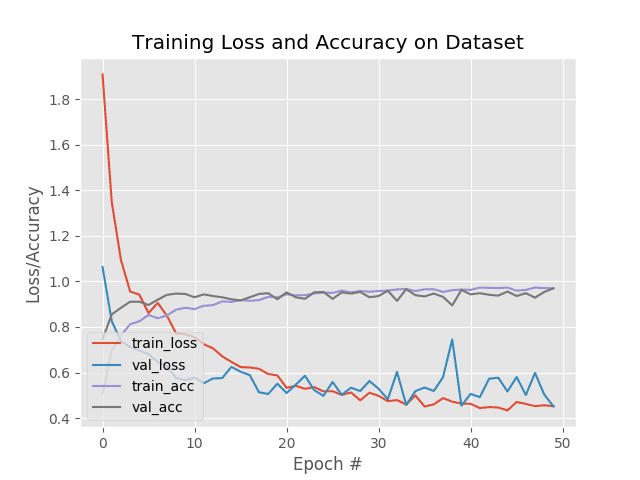 Figure 13: My accuracy/loss plot generated with Keras and matplotlib for training StridedNet, an example CNN to showcase Keras Conv2D parameters.
As you can see, our network is obtaining ~97% accuracy on the testing set with minimal overfitting!
You can apply deep learning to your own projects
You don’t need a degree in computer science or mathematics to study deep learning.
Instead, what you need is a book that is designed with the practitioner in mind — a book that not only teaches you the theory of how and why deep learning algorithms work, but then takes that theory and implements it in code so you fully understand it.
Sound too good to be true?
It’s not.
Inside my book, Deep Learning for Computer Vision with Python, you’ll find over 900+ pages of the most complete, comprehensive computer vision and deep learning education available online.
Regardless of whether you’re just getting started in deep learning or you’re already a seasoned deep learning practitioner, my book will help you master computer vision and deep learning through:
-
Super practical walkthroughs that present solutions to actual, real-world problems through image classification (ResNet, Inception, etc.), object detection (Faster R-CNN, SSDs, RetinaNet), and instance segmentation (Mask R-CNNs).
-
Hands-on tutorials (with lots of code) that not only show you the algorithms behind deep learning for computer vision but their implementations as well.
-
A no-nonsense teaching style that is guaranteed to help you master deep learning for image understanding and visual recognition.
But don’t take my word for it — Deep Learning for Computer Vision with Python is trusted by members of major universities and corporations. It has helped them on their journey to CV/DL mastery and I have no doubt it will help you too.
To learn more (and grab your free table of contents + sample chapters PDF), just use the link below:
Grab your free table of contents + sample chapters
Summary
In today’s tutorial, we discussed convolutional layers and the Keras Conv2D class.
You now know:
What the most important parameters are to the Keras Conv2D class ( filters , kernel_size , strides , padding )
-
What proper values are for these parameters
-
How to use the Keras Conv2D class to create your own Convolutional Neural Network
-
How to train your CNN and evaluate it on an example dataset
I hope you found this tutorial helpful in understanding the parameters to Keras’ Conv2D Class — if you did, please leave a comment in the comments section.
If you would like to download the source code to this blog post (and to be notified when future tutorials are published here on PyImageSearch), just enter your email address in the form below.