Mask R-CNN with OpenCV

In this tutorial, you will learn how to use Mask R-CNN with OpenCV.

Using Mask R-CNN you can automatically segment and construct pixel-wise masks for every object in an image. We’ll be applying Mask R-CNNs to both images and video streams.

In last week’s blog post you learned how to use the YOLO object detector to detect the presence of objects in images. Object detectors, such as YOLO, Faster R-CNNs, and Single Shot Detectors (SSDs), generate four sets of (x, y)-coordinates which represent the bounding box of an object in an image.

Obtaining the bounding boxes of an object is a good start but the bounding box itself doesn’t tell us anything about (1) which pixels belong to the foreground object and (2) which pixels belong to the background.

That begs the question:

Is it possible to generate a mask for each object in our image, thereby allowing us to segment the foreground object from the background? Is such a method even possible?

The answer is yes — we just need to perform instance segmentation using the Mask R-CNN architecture.

To learn how to apply Mask R-CNN with OpenCV to both images and video streams, just keep reading!

Mask R-CNN with OpenCV

In the first part of this tutorial, we’ll discuss the difference between image classification, object detection, instance segmentation, and semantic segmentation.

From there we’ll briefly review the Mask R-CNN architecture and its connections to Faster R-CNN.

I’ll then show you how to apply Mask R-CNN with OpenCV to both images and video streams.

Let’s get started!

Instance segmentation vs. Semantic segmentation

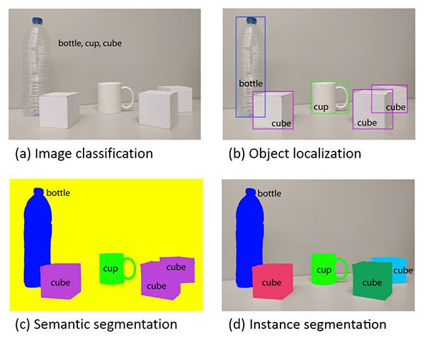
Figure 1: Image classification (top-left), object detection (top-right), semantic segmentation (bottom-left), and instance segmentation (bottom-right). We’ll be performing instance segmentation with Mask R-CNN in this tutorial. (source)

Explaining the differences between traditional image classification, object detection, semantic segmentation, and instance segmentation is best done visually.

When performing traditional image classification our goal is to predict a set of labels to characterize the contents of an input image (top-left).

Object detection builds on image classification, but this time allows us to localize each object in an image. The image is now characterized by:

1. Bounding box (x, y)-coordinates for each object

2. An associated class label for each bounding box

An example of semantic segmentation can be seen in bottom-left. Semantic segmentation algorithms require us to associate every pixel in an input image with a class label (including a class label for the background).

Pay close attention to our semantic segmentation visualization — notice how each object is indeed segmented but each “cubeâ€� object has the same color.

While semantic segmentation algorithms are capable of labeling every object in an image they cannot differentiate between two objects of the same class.

This behavior is especially problematic if two objects of the same class are partially occluding each other — we have no idea where the boundaries of one object ends and the next one begins, as demonstrated by the two purple cubes, we cannot tell where one cube starts and the other ends.

Instance segmentation algorithms, on the other hand, compute a pixel-wise mask for every object in the image, even if the objects are of the same class label (bottom-right). Here you can see that each of the cubes has their own unique color, implying that our instance segmentation algorithm not only localized each individual cube but predicted their boundaries as well.

The Mask R-CNN architecture we’ll be discussing in this tutorial is an example of an instance segmentation algorithm.

What is Mask R-CNN?

The Mask R-CNN algorithm was introduced by He et al. in their 2017 paper, Mask R-CNN.

Mask R-CNN builds on the previous object detection work of R-CNN (2013), Fast R-CNN (2015), and Faster R-CNN (2015), all by Girshick et al.

In order to understand Mask R-CNN let’s briefly review the R-CNN variants, starting with the original R-CNN:

The original R-CNN algorithm is a four-step process:

• Step #1: Input an image to the network.

• Step #2: Extract region proposals (i.e., regions of an image that potentially contain objects) using an algorithm such as Selective Search.

• Step #3: Use transfer learning, specifically feature extraction, to compute features for each proposal (which is effectively an ROI) using the pre-trained CNN.

• Step #4: Classify each proposal using the extracted features with a Support Vector Machine (SVM).

The reason this method works is due to the robust, discriminative features learned by the CNN.

However, the problem with the R-CNN method is it’s incredibly slow. And furthermore, we’re not actually learning to localize via a deep neural network, we’re effectively just building a more advanced HOG + Linear SVM detector.

To improve upon the original R-CNN, Girshick et al. published the Fast R-CNN algorithm:

Similar to the original R-CNN, Fast R-CNN still utilizes Selective Search to obtain region proposals; however, the novel contribution from the paper was Region of Interest (ROI) Pooling module.

ROI Pooling works by extracting a fixed-size window from the feature map and using these features to obtain the final class label and bounding box. The primary benefit here is that the network is now, effectively, end-to-end trainable:

1. We input an image and associated ground-truth bounding boxes

2. Extract the feature map

3. Apply ROI pooling and obtain the ROI feature vector

4. And finally, use the two sets of fully-connected layers to obtain (1) the class label predictions and (2) the bounding box locations for each proposal.

While the network is now end-to-end trainable, performance suffered dramatically at inference (i.e., prediction) by being dependent on Selective Search.

To make the R-CNN architecture even faster we need to incorporate the region proposal directly into the R-CNN:

The Faster R-CNN paper by Girshick et al. introduced the Region Proposal Network (RPN) that bakes region proposal directly into the architecture, alleviating the need for the Selective Search algorithm.

As a whole, the Faster R-CNN architecture is capable of running at approximately 7-10 FPS, a huge step towards making real-time object detection with deep learning a reality.

The Mask R-CNN algorithm builds on the Faster R-CNN architecture with two major contributions:

1. Replacing the ROI Pooling module with a more accurate ROI Align module

2. Inserting an additional branch out of the ROI Align module

This additional branch accepts the output of the ROI Align and then feeds it into two CONV layers.

The output of the CONV layers is the mask itself.

We can visualize the Mask R-CNN architecture in the following figure:

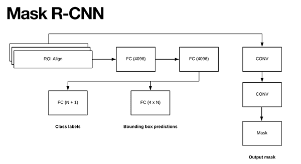
Figure 5: The Mask R-CNN work by He et al. replaces the ROI Polling module with a more accurate ROI Align module. The output of the ROI module is then fed into two CONV layers. The output of the CONV layers is the mask itself.

Notice the branch of two CONV layers coming out of the ROI Align module — this is where our mask is actually generated.

As we know, the Faster R-CNN/Mask R-CNN architectures leverage a Region Proposal Network (RPN) to generate regions of an image that potentially contain an object.

Each of these regions is ranked based on their “objectness score� (i.e., how likely it is that a given region could potentially contain an object) and then the top N most confident objectness regions are kept.

In the original Faster R-CNN publication Girshick et al. set N=2,000, but in practice, we can get away with a much smaller N, such as N={10, 100, 200, 300} and still obtain good results.

He et al. set N=300 in their publication which is the value we’ll use here as well.

Each of the 300 selected ROIs go through three parallel branches of the network:

1. Label prediction

2. Bounding box prediction

3. Mask prediction

Figure 5 above above visualizes these branches.

During prediction, each of the 300 ROIs go through non-maxima suppression and the top 100 detection boxes are kept, resulting in a 4D tensor of 100 x L x 15 x 15 where L is the number of class labels in the dataset and 15 x 15 is the size of each of the L masks.

The Mask R-CNN we’re using here today was trained on the COCO dataset, which has L=90 classes, thus the resulting volume size from the mask module of the Mask R CNN is 100 x 90 x 15 x 15.

To visualize the Mask R-CNN process take a look at the figure below:

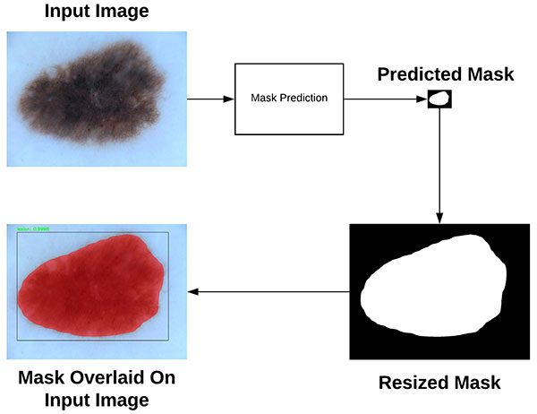
Figure 6: A visualization of Mask R-CNN producing a 15 x 15 mask, the mask resized to the original dimensions of the image, and then finally overlaying the mask on the original image. (source: Deep Learning for Computer Vision with Python, ImageNet Bundle)

Here you can see that we start with our input image and feed it through our Mask R-CNN network to obtain our mask prediction.

The predicted mask is only 15 x 15 pixels so we resize the mask back to the original input image dimensions.

Finally, the resized mask can be overlaid on the original input image. For a more thorough discussion on how Mask R-CNN works be sure to refer to:

1. The original Mask R-CNN publication by He et al.

2. My book, Deep Learning for Computer Vision with Python, where I discuss Mask R-CNNs in more detail, including how to train your own Mask R-CNNs from scratch on your own data.

Project structure

Our project today consists of two scripts, but there are several other files that are important.

I’ve organized the project in the following manner (as is shown by the tree command output directly in a terminal):

12345678910111213141516171819

$ tree.├── mask-rcnn-coco│ ├── colors.txt│ ├── frozen_inference_graph.pb│ ├── mask_rcnn_inception_v2_coco_2018_01_28.pbtxt│ └── object_detection_classes_coco.txt├── images│ ├── example_01.jpg│ ├── example_02.jpg│ └── example_03.jpg├── videos│ ├── ├── output│ ├──  â”œâ”€â”€ mask_rcnn.py└── mask_rcnn_video.py 4 directories, 9 files

2

4

6

8

10

12

14

16

18

.

│ ├── colors.txt

│ ├── mask_rcnn_inception_v2_coco_2018_01_28.pbtxt

├── images

│ ├── example_02.jpg

├── videos

├── output

├── mask_rcnn.py

 

Our project consists of four directories:

mask-rcnn-coco/ : The Mask R-CNN model files. There are four files:

frozen_inference_graph.pb : The Mask R-CNN model weights. The weights are pre-trained on the COCO dataset.

mask_rcnn_inception_v2_coco_2018_01_28.pbtxt : The Mask R-CNN model configuration. If you’d like to build + train your own model on your own annotated data, refer to Deep Learning for Computer Vision with Python.

object_detection_classes_coco.txt : All 90 classes are listed in this text file, one per line. Open it in a text editor to see what objects our model can recognize.

colors.txt : This text file contains six colors to randomly assign to objects found in the image.

We’ll be reviewing two scripts today:

mask_rcnn.py : This script will perform instance segmentation and apply a mask to the image so you can see where, down to the pixel, the Mask R-CNN thinks an object is.

mask_rcnn_video.py : This video processing script uses the same Mask R-CNN and applies the model to every frame of a video file. The script then writes the output frame back to a video file on disk.

OpenCV and Mask R-CNN in images

Now that we’ve reviewed how Mask R-CNNs work, let’s get our hands dirty with some Python code.

Before we begin, ensure that your Python environment has OpenCV 3.4.2/3.4.3 or higher installed. You can follow one of my OpenCV installation tutorials to upgrade/install OpenCV. If you want to be up and running in 5 minutes or less, you can consider installing OpenCV with pip. If you have some other requirements, you might want to compile OpenCV from source.

Make sure you’ve used the “Downloads� section of this blog post to download the source code, trained Mask R-CNN, and example images.

From there, open up the mask_rcnn.py file and insert the following code:

# import the necessary packagesimport numpy as npimport argparseimport randomimport timeimport cv2import os

import numpy as np

import random

import cv2

First we’ll import our required packages on Lines 2-7. Notably, we’re importing NumPy and OpenCV. Everything else comes with most Python installations.

From there, we’ll parse our command line arguments:

9101112131415161718192021

# construct the argument parse and parse the argumentsap = argparse.ArgumentParser()ap.add_argument(“-i”, “–image”, required=True, help=”path to input image”)ap.add_argument(“-m”, “–mask-rcnn”, required=True, help=”base path to mask-rcnn directory”)ap.add_argument(“-v”, “–visualize”, type=int, default=0, help=”whether or not we are going to visualize each instance”)ap.add_argument(“-c”, “–confidence”, type=float, default=0.5, help=”minimum probability to filter weak detections”)ap.add_argument(“-t”, “–threshold”, type=float, default=0.3, help=”minimum threshold for pixel-wise mask segmentation”)args = vars(ap.parse_args())

10

12

14

16

18

20

ap = argparse.ArgumentParser()

help=”path to input image”)

help=”base path to mask-rcnn directory”)

help=”whether or not we are going to visualize each instance”)

help=”minimum probability to filter weak detections”)

help=”minimum threshold for pixel-wise mask segmentation”)

Our script requires that command line argument flags and parameters be passed at runtime in our terminal. Our arguments are parsed on Lines 10-21, where the first two of the following are required and the rest are optional:

–image : The path to our input image.

–mask-rnn : The base path to the Mask R-CNN files.

–visualize (optional): A positive value indicates that we want to visualize how we extracted the masked region on our screen. Either way, we’ll display the final output on the screen.

–confidence (optional): You can override the probability value of 0.5 which serves to filter weak detections.

–threshold (optional): We’ll be creating a binary mask for each object in the image and this threshold value will help us filter out weak mask predictions. I found that a default value of 0.3 works pretty well.

Now that our command line arguments are stored in the args dictionary, let’s load our labels and colors:

# load the COCO class labels our Mask R-CNN was trained onlabelsPath = os.path.sep.join([args[“mask_rcnn”], “object_detection_classes_coco.txt”])LABELS = open(labelsPath).read().strip().split(“\n”) # load the set of colors that will be used when visualizing a given# instance segmentationcolorsPath = os.path.sep.join([args[“mask_rcnn”], “colors.txt”])COLORS = open(colorsPath).read().strip().split(“\n”)COLORS = [np.array(c.split(“,”)).astype(“int”) for c in COLORS]COLORS = np.array(COLORS, dtype=”uint8”)

labelsPath = os.path.sep.join([args[“mask_rcnn”],

LABELS = open(labelsPath).read().strip().split(“\n”)

load the set of colors that will be used when visualizing a given

colorsPath = os.path.sep.join([args[“mask_rcnn”], “colors.txt”])

COLORS = [np.array(c.split(“,”)).astype(“int”) for c in COLORS]

Lines 24-26 load the COCO object class LABELS . Today’s Mask R-CNN is capable of recognizing 90 classes including people, vehicles, signs, animals, everyday items, sports gear, kitchen items, food, and more! I encourage you to look at object_detection_classes_coco.txt to see the available classes.

From there we load the COLORS from the path, performing a couple array conversion operations (Lines 30-33).

Let’s load our model:

# derive the paths to the Mask R-CNN weights and model configurationweightsPath = os.path.sep.join([args[“mask_rcnn”], “frozen_inference_graph.pb”])configPath = os.path.sep.join([args[“mask_rcnn”], “mask_rcnn_inception_v2_coco_2018_01_28.pbtxt”]) # load our Mask R-CNN trained on the COCO dataset (90 classes)# from diskprint(“[INFO] loading Mask R-CNN from disk…“)net = cv2.dnn.readNetFromTensorflow(weightsPath, configPath)

weightsPath = os.path.sep.join([args[“mask_rcnn”],

configPath = os.path.sep.join([args[“mask_rcnn”],

 

from disk

net = cv2.dnn.readNetFromTensorflow(weightsPath, configPath)

First, we build our weight and configuration paths (Lines 36-39), followed by loading the model via these paths (Line 44).

In the next block, we’ll load and pass an image through the Mask R-CNN neural net:

464748495051525354555657585960616263

# load our input image and grab its spatial dimensionsimage = cv2.imread(args[“image”])(H, W) = image.shape[:2] # construct a blob from the input image and then perform a forward# pass of the Mask R-CNN, giving us (1) the bounding box  coordinates# of the objects in the image along with (2) the pixel-wise segmentation# for each specific objectblob = cv2.dnn.blobFromImage(image, swapRB=True, crop=False)net.setInput(blob)start = time.time()(boxes, masks) = net.forward([“detection_out_final”, “detection_masks”])end = time.time() # show timing information and volume information on Mask R-CNNprint(“[INFO] Mask R-CNN took {:.6f} seconds”.format(end - start))print(“[INFO] boxes shape: {}”.format(boxes.shape))print(“[INFO] masks shape: {}”.format(masks.shape))

47

49

51

53

55

57

59

61

63

image = cv2.imread(args[“image”])

 

pass of the Mask R-CNN, giving us (1) the bounding box  coordinates

for each specific object

net.setInput(blob)

(boxes, masks) = net.forward([“detection_out_final”, “detection_masks”])

 

print(“[INFO] Mask R-CNN took {:.6f} seconds”.format(end - start))

print(“[INFO] masks shape: {}”.format(masks.shape))

Here we:

Load the input image and extract dimensions for scaling purposes later (Lines 47 and 48). Construct a blob via cv2.dnn.blobFromImage (Line 54). You can learn why and how to use this function in my previous tutorial. Perform a forward pass of the blob through the net while collecting timestamps (Lines 55-58). The results are contained in two important variables: boxes and masks .

Now that we’ve performed a forward pass of the Mask R-CNN on the image, we’ll want to filter + visualize our results. That’s exactly what this next for loop accomplishes. It is quite long, so I’ve broken it into five code blocks beginning here:

6566676869707172737475767778798081828384

# loop over the number of detected objectsfor i in range(0, boxes.shape[2]): # extract the class ID of the detection along with the confidence # (i.e., probability) associated with the prediction classID = int(boxes[0, 0, i, 1]) confidence = boxes[0, 0, i, 2]  # filter out weak predictions by ensuring the detected probability # is greater than the minimum probability if confidence > args[“confidence”]: # clone our original image so we can draw on it clone = image.copy()  # scale the bounding box coordinates back relative to the # size of the image and then compute the width and the height # of the bounding box box = boxes[0, 0, i, 3:7] * np.array([W, H, W, H]) (startX, startY, endX, endY) = box.astype(“int”) boxW = endX - startX boxH = endY - startY

66

68

70

72

74

76

78

80

82

84

for i in range(0, boxes.shape[2]):

# (i.e., probability) associated with the prediction

confidence = boxes[0, 0, i, 2]

# filter out weak predictions by ensuring the detected probability

if confidence > args[“confidence”]:

clone = image.copy()

# scale the bounding box coordinates back relative to the

# of the bounding box

(startX, startY, endX, endY) = box.astype(“int”)

boxH = endY - startY

In this block, we begin our filter/visualization loop (Line 66).

We proceed to extract the classID and confidence of a particular detected object (Lines 69 and 70).

From there we filter out weak predictions by comparing the confidence to the command line argument confidence value, ensuring we exceed it (Line 74).

Assuming that’s the case, we’ll go ahead and make a clone of the image (Line 76). We’ll need this image later.

Then we scale our object’s bounding box as well as calculate the box dimensions (Lines 81-84).

Image segmentation requires that we find all pixels where an object is present. Thus, we’re going to place a transparent overlay on top of the object to see how well our algorithm is performing. In order to do so, we’ll calculate a mask:

# extract the pixel-wise segmentation for the object, resize # the mask such that it’s the same dimensions of the bounding # box, and then finally threshold to create a binary mask mask = masks[i, classID] mask = cv2.resize(mask, (boxW, boxH), interpolation=cv2.INTER_NEAREST) mask = (mask > args[“threshold”])  # extract the ROI of the image roi = clone[startY:endY, startX:endX]

# the mask such that it’s the same dimensions of the bounding

mask = masks[i, classID]

interpolation=cv2.INTER_NEAREST)

 

roi = clone[startY:endY, startX:endX]

On Lines 89-91, we extract the pixel-wise segmentation for the object as well as resize it to the original image dimensions. Finally we threshold the mask so that it is a binary array/image (Line 92).

We also extract the region of interest where the object resides (Line 95).

Both the mask and roi can be seen visually in Figure 8 later in the post.

For convenience, this next block accomplishes visualizing the mask , roi , and segmented instance if the –visualize flag is set via command line arguments:

979899100101102103104105106107108109

# check to see if are going to visualize how to extract the # masked region itself if args[“visualize”] > 0: # convert the mask from a boolean to an integer mask with # to values: 0 or 255, then apply the mask visMask = (mask * 255).astype(“uint8”) instance = cv2.bitwise_and(roi, roi, mask=visMask)  # show the extracted ROI, the mask, along with the # segmented instance cv2.imshow(“ROI”, roi) cv2.imshow(“Mask”, visMask) cv2.imshow(“Segmented”, instance)

98

100

102

104

106

108

# masked region itself

# convert the mask from a boolean to an integer mask with

visMask = (mask * 255).astype(“uint8”)

 

# segmented instance

cv2.imshow(“Mask”, visMask)

In this block we:

• Check to see if we should visualize the ROI, mask, and segmented instance (Line 99).

• Convert our mask from boolean to integer where a value of “0” indicates background and “255” foreground (Line 102).

• Perform bitwise masking to visualize just the instance itself (Line 103).

• Show all three images (Lines 107-109).

Again, these visualization images will only be shown if the –visualize flag is set via the optional command line argument (by default these images won’t be shown).

Now let’s continue on with visualization:

111112113114115116117118119120121122

# now, extract only the masked region of the ROI by passing # in the boolean mask array as our slice condition roi = roi[mask]  # randomly select a color that will be used to visualize this # particular instance segmentation then create a transparent # overlay by blending the randomly selected color with the ROI color = random.choice(COLORS) blended = ((0.4 * color) + (0.6 * roi)).astype(“uint8”)  # store the blended ROI in the original image clone[startY:endY, startX:endX][mask] = blended

112

114

116

118

120

122

# in the boolean mask array as our slice condition

 

# particular instance segmentation then create a transparent

color = random.choice(COLORS)

 

clone[startY:endY, startX:endX][mask] = blended

Line 113 extracts only the masked region of the ROI by passing the boolean mask array as our slice condition.

Then we’ll randomly select one of our six COLORS to apply our transparent overlay on the object (Line 118).

Subsequently, we’ll blend our masked region with the roi (Line 119) followed by placing this blended region into the clone image (Line 122).

Finally, we’ll draw the rectangle and textual class label + confidence value on the image as well as display the result!

124125126127128129130131132133134135136

# draw the bounding box of the instance on the image color = [int(c) for c in color] cv2.rectangle(clone, (startX, startY), (endX, endY), color, 2)  # draw the predicted label and associated probability of the # instance segmentation on the image text = “{}: {:.4f}”.format(LABELS[classID], confidence) cv2.putText(clone, text, (startX, startY - 5), cv2.FONT_HERSHEY_SIMPLEX, 0.5, color, 2)  # show the output image cv2.imshow(“Output”, clone) cv2.waitKey(0)

125

127

129

131

133

135

color = [int(c) for c in color]

 

# instance segmentation on the image

cv2.putText(clone, text, (startX, startY - 5),

 

cv2.imshow(“Output”, clone)

To close out, we:

• Draw a colored bounding box around the object (Lines 125 and 126).

Build our class label + confidence text as well as draw the text above the bounding box (Lines 130-132).

• Display the image until any key is pressed (Lines 135 and 136).

Let’s give our Mask R-CNN code a try!

Make sure you’ve used the “Downloads� section of the tutorial to download the source code, trained Mask R-CNN, and example images. From there, open up your terminal and execute the following command:

$ python mask_rcnn.py –mask-rcnn mask-rcnn-coco –image images/example_01.jpg[INFO] loading Mask R-CNN from disk…[INFO] Mask R-CNN took 0.761193 seconds[INFO] boxes shape: (1, 1, 3, 7)[INFO] masks shape: (100, 90, 15, 15)

[INFO] loading Mask R-CNN from disk…

[INFO] boxes shape: (1, 1, 3, 7)

Figure 7: A Mask R-CNN applied to a scene of cars. Python and OpenCV were used to generate the masks.

In the above image, you can see that our Mask R-CNN has not only localized each of the cars in the image but has also constructed a pixel-wise mask as well, allowing us to segment each car from the image.

If we were to run the same command, this time supplying the –visualize flag, we can visualize the ROI, mask, and instance as well:

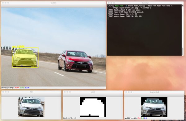
Figure 8: Using the --visualize flag, we can view the ROI, mask, and segmentmentation intermediate steps for our Mask R-CNN pipeline built with Python and OpenCV.

Let’s try another example image:

$ python mask_rcnn.py –mask-rcnn mask-rcnn-coco –image images/example_02.jpg \ –confidence 0.6[INFO] loading Mask R-CNN from disk…[INFO] Mask R-CNN took 0.676008 seconds[INFO] boxes shape: (1, 1, 8, 7)[INFO] masks shape: (100, 90, 15, 15)

–confidence 0.6

[INFO] Mask R-CNN took 0.676008 seconds

[INFO] masks shape: (100, 90, 15, 15)

Figure 9: Using Python and OpenCV, we can perform instance segmentation using a Mask R-CNN.

Our Mask R-CNN has correctly detected and segmented both people, a dog, a horse, and a truck from the image.

Here’s one final example before we move on to using Mask R-CNNs in videos:

$ python mask_rcnn.py –mask-rcnn mask-rcnn-coco –image images/example_03.jpg [INFO] loading Mask R-CNN from disk…[INFO] Mask R-CNN took 0.680739 seconds[INFO] boxes shape: (1, 1, 3, 7)[INFO] masks shape: (100, 90, 15, 15)

[INFO] loading Mask R-CNN from disk…

[INFO] boxes shape: (1, 1, 3, 7)

Figure 10: Here you can see me feeding a treat to the family beagle, Jemma. The pixel-wise map of each object identified is masked and transparently overlaid on the objects. This image was generated with OpenCV and Python using a pre-trained Mask R-CNN model.

In this image, you can see a photo of myself and Jemma, the family beagle.

Our Mask R-CNN is capable of detecting and localizing me, Jemma, and the chair with high confidence.

OpenCV and Mask R-CNN in video streams

Now that we’ve looked at how to apply Mask R-CNNs to images, let’s explore how they can be applied to videos as well.

Open up the mask_rcnn_video.py file and insert the following code:

123456789101112131415161718192021

# import the necessary packagesimport numpy as npimport argparseimport imutilsimport timeimport cv2import os # construct the argument parse and parse the argumentsap = argparse.ArgumentParser()ap.add_argument(“-i”, “–input”, required=True, help=”path to input video file”)ap.add_argument(“-o”, “–output”, required=True, help=”path to output video file”)ap.add_argument(“-m”, “–mask-rcnn”, required=True, help=”base path to mask-rcnn directory”)ap.add_argument(“-c”, “–confidence”, type=float, default=0.5, help=”minimum probability to filter weak detections”)ap.add_argument(“-t”, “–threshold”, type=float, default=0.3, help=”minimum threshold for pixel-wise mask segmentation”)args = vars(ap.parse_args())

2

4

6

8

10

12

14

16

18

20

import numpy as np

import imutils

import cv2

 

ap = argparse.ArgumentParser()

help=”path to input video file”)

help=”path to output video file”)

help=”base path to mask-rcnn directory”)

help=”minimum probability to filter weak detections”)

help=”minimum threshold for pixel-wise mask segmentation”)

First we import our necessary packages and parse our command line arguments.

There are two new command line arguments (which replaces –image from the previous script):

–input : The path to our input video.

–output : The path to our output video (since we’ll be writing our results to disk in a video file).

Now let’s load our class LABELS , COLORS , and Mask R-CNN neural net :

2324252627282930313233343536373839404142

# load the COCO class labels our Mask R-CNN was trained onlabelsPath = os.path.sep.join([args[“mask_rcnn”], “object_detection_classes_coco.txt”])LABELS = open(labelsPath).read().strip().split(“\n”) # initialize a list of colors to represent each possible class labelnp.random.seed(42)COLORS = np.random.randint(0, 255, size=(len(LABELS), 3), dtype=”uint8”) # derive the paths to the Mask R-CNN weights and model configurationweightsPath = os.path.sep.join([args[“mask_rcnn”], “frozen_inference_graph.pb”])configPath = os.path.sep.join([args[“mask_rcnn”], “mask_rcnn_inception_v2_coco_2018_01_28.pbtxt”]) # load our Mask R-CNN trained on the COCO dataset (90 classes)# from diskprint(“[INFO] loading Mask R-CNN from disk…“)net = cv2.dnn.readNetFromTensorflow(weightsPath, configPath)

24

26

28

30

32

34

36

38

40

42

labelsPath = os.path.sep.join([args[“mask_rcnn”],

LABELS = open(labelsPath).read().strip().split(“\n”)

initialize a list of colors to represent each possible class label

COLORS = np.random.randint(0, 255, size=(len(LABELS), 3),

 

weightsPath = os.path.sep.join([args[“mask_rcnn”],

configPath = os.path.sep.join([args[“mask_rcnn”],

 

from disk

net = cv2.dnn.readNetFromTensorflow(weightsPath, configPath)

Our LABELS and COLORS are loaded on Lines 24-31.

From there we define our weightsPath and configPath before loading our Mask R-CNN neural net (Lines 34-42).

Now let’s initialize our video stream and video writer:

44454647484950515253545556575859

# initialize the video stream and pointer to output video filevs = cv2.VideoCapture(args[“input”])writer = None # try to determine the total number of frames in the video filetry: prop = cv2.cv.CV_CAP_PROP_FRAME_COUNT if imutils.is_cv2() \ else cv2.CAP_PROP_FRAME_COUNT total = int(vs.get(prop)) print(“[INFO] {} total frames in video”.format(total)) # an error occurred while trying to determine the total# number of frames in the video fileexcept: print(“[INFO] could not determine # of frames in video”) total = -1

45

47

49

51

53

55

57

59

vs = cv2.VideoCapture(args[“input”])

 

try:

else cv2.CAP_PROP_FRAME_COUNT

print(“[INFO] {} total frames in video”.format(total))

an error occurred while trying to determine the total

except:

total = -1

Our video stream ( vs ) and video writer are initialized on Lines 45 and 46.

We attempt to determine the number of frames in the video file and display the total (Lines 49-53). If we’re unsuccessful, we’ll capture the exception and print a status message as well as set total to -1 (Lines 57-59). We’ll use this value to approximate how long it will take to process an entire video file.

Let’s begin our frame processing loop:

6162636465666768697071727374757677787980

# loop over frames from the video file streamwhile True: # read the next frame from the file (grabbed, frame) = vs.read()  # if the frame was not grabbed, then we have reached the end # of the stream if not grabbed: break  # construct a blob from the input frame and then perform a # forward pass of the Mask R-CNN, giving us (1) the bounding box # coordinates of the objects in the image along with (2) the # pixel-wise segmentation for each specific object blob = cv2.dnn.blobFromImage(frame, swapRB=True, crop=False) net.setInput(blob) start = time.time() (boxes, masks) = net.forward([“detection_out_final”, “detection_masks”]) end = time.time()

62

64

66

68

70

72

74

76

78

80

while True:

(grabbed, frame) = vs.read()

# if the frame was not grabbed, then we have reached the end

if not grabbed:

 

# forward pass of the Mask R-CNN, giving us (1) the bounding box

# pixel-wise segmentation for each specific object

net.setInput(blob)

(boxes, masks) = net.forward([“detection_out_final”,

end = time.time()

We begin looping over frames by defining an infinite while loop and capturing the first frame (Lines 62-64). The loop will process the video until completion which is handled by the exit condition on Lines 68 and 69.

We then construct a blob from the frame and pass it through the neural net while grabbing the elapsed time so we can calculate estimated time to completion later (Lines 75-80). The result is included in both boxes and masks .

Now let’s begin looping over detected objects:

828384858687888990919293949596979899100101102103104105106107108109110111112113

# loop over the number of detected objects for i in range(0, boxes.shape[2]): # extract the class ID of the detection along with the # confidence (i.e., probability) associated with the # prediction classID = int(boxes[0, 0, i, 1]) confidence = boxes[0, 0, i, 2]  # filter out weak predictions by ensuring the detected # probability is greater than the minimum probability if confidence > args[“confidence”]: # scale the bounding box coordinates back relative to the # size of the frame and then compute the width and the # height of the bounding box (H, W) = frame.shape[:2] box = boxes[0, 0, i, 3:7] * np.array([W, H, W, H]) (startX, startY, endX, endY) = box.astype(“int”) boxW = endX - startX boxH = endY - startY  # extract the pixel-wise segmentation for the object, # resize the mask such that it’s the same dimensions of # the bounding box, and then finally threshold to create # a binary mask mask = masks[i, classID] mask = cv2.resize(mask, (boxW, boxH), interpolation=cv2.INTER_NEAREST) mask = (mask > args[“threshold”])  # extract the ROI of the image but only extracted the # masked region of the ROI roi = frame[startY:endY, startX:endX][mask]

83

85

87

89

91

93

95

97

99

101

103

105

107

109

111

113

for i in range(0, boxes.shape[2]):

# confidence (i.e., probability) associated with the

classID = int(boxes[0, 0, i, 1])

 

# probability is greater than the minimum probability

# scale the bounding box coordinates back relative to the

# height of the bounding box

box = boxes[0, 0, i, 3:7] * np.array([W, H, W, H])

boxW = endX - startX

 

# resize the mask such that it’s the same dimensions of

# a binary mask

mask = cv2.resize(mask, (boxW, boxH),

mask = (mask > args[“threshold”])

# extract the ROI of the image but only extracted the

roi = frame[startY:endY, startX:endX][mask]

First we filter out weak detections with a low confidence value. Then we determine the bounding box coordinates and obtain the mask and roi .

Now let’s draw the object’s transparent overlay, bounding rectangle, and label + confidence:

115116117118119120121122123124125126127128129130131132133

# grab the color used to visualize this particular class, # then create a transparent overlay by blending the color # with the ROI color = COLORS[classID] blended = ((0.4 * color) + (0.6 * roi)).astype(“uint8”)  # store the blended ROI in the original frame frame[startY:endY, startX:endX][mask] = blended  # draw the bounding box of the instance on the frame color = [int(c) for c in color] cv2.rectangle(frame, (startX, startY), (endX, endY), color, 2)  # draw the predicted label and associated probability of # the instance segmentation on the frame text = “{}: {:.4f}”.format(LABELS[classID], confidence) cv2.putText(frame, text, (startX, startY - 5), cv2.FONT_HERSHEY_SIMPLEX, 0.5, color, 2)

116

118

120

122

124

126

128

130

132

# then create a transparent overlay by blending the color

color = COLORS[classID]

 

frame[startY:endY, startX:endX][mask] = blended

# draw the bounding box of the instance on the frame

cv2.rectangle(frame, (startX, startY), (endX, endY),

 

# the instance segmentation on the frame

cv2.putText(frame, text, (startX, startY - 5),

Here we’ve blended our roi with color and store it in the original frame , effectively creating a colored transparent overlay (Lines 118-122).

We then draw a rectangle around the object and display the class label + confidence just above (Lines 125-133).

Finally, let’s write to the video file and clean up:

135136137138139140141142143144145146147148149150151152153154155

# check if the video writer is None if writer is None: # initialize our video writer fourcc = cv2.VideoWriter_fourcc(*“MJPG”) writer = cv2.VideoWriter(args[“output”], fourcc, 30, (frame.shape[1], frame.shape[0]), True)  # some information on processing single frame if total > 0: elap = (end - start) print(“[INFO] single frame took {:.4f} seconds”.format(elap)) print(“[INFO] estimated total time to finish: {:.4f}”.format( elap * total))  # write the output frame to disk writer.write(frame) # release the file pointersprint(“[INFO] cleaning up…“)writer.release()vs.release()

136

138

140

142

144

146

148

150

152

154

if writer is None:

fourcc = cv2.VideoWriter_fourcc(*“MJPG”)

(frame.shape[1], frame.shape[0]), True)

# some information on processing single frame

elap = (end - start)

print(“[INFO] estimated total time to finish: {:.4f}”.format(

 

writer.write(frame)

release the file pointers

writer.release()

On the first iteration of the loop, our video writer is initialized.

An estimate of the amount of time that the processing will take is printed to the terminal on Lines 143-147.

The final operation of our loop is to write the frame to disk via our writer object (Line 150).

You’ll notice that I’m not displaying each frame to the screen. The display operation is time-consuming and you’ll be able to view the output video with any media player when the script is finished processing anyways.

Note: Furthermore, OpenCV does not support NVIDIA GPUs for it’s dnn module. Right now only a limited number of GPUs are supported, mainly Intel GPUs. NVIDIA GPU support is coming soon but for the time being we cannot easily use a GPU with OpenCV’s dnn module.

Lastly, we release video input and output file pointers (Lines 154 and 155).

Now that we’ve coded up our Mask R-CNN + OpenCV script for video streams, let’s give it a try!

Make sure you use the “Downloads� section of this tutorial to download the source code and Mask R-CNN model.

You’ll then need to collect your own videos with your smartphone or another recording device. Alternatively, you can download videos from YouTube as I have done.

Note: I am intentionally not including the videos in today’s download because they are rather large (400MB+). If you choose to use the same videos as me, the credits and links are at the bottom of this section.

From there, open up a terminal and execute the following command:

$ python mask_rcnn_video.py –input videos/cats_and_dogs.mp4 \ –output output/cats_and_dogs_output.avi –mask-rcnn mask-rcnn-coco[INFO] loading Mask R-CNN from disk…[INFO] 19312 total frames in video[INFO] single frame took 0.8585 seconds[INFO] estimated total time to finish: 16579.2047

–output output/cats_and_dogs_output.avi –mask-rcnn mask-rcnn-coco

[INFO] 19312 total frames in video

[INFO] estimated total time to finish: 16579.2047

Figure 11: Mask R-CNN applied to video with Python and OpenCV.

In the above video, you can find funny video clips of dogs and cats with a Mask R-CNN applied to them!

Here is a second example, this one of applying OpenCV and a Mask R- CNN to video clips of cars “slipping and sliding� in wintry conditions:

$ python mask_rcnn_video.py –input videos/slip_and_slide.mp4 \ –output output/slip_and_slide_output.avi –mask-rcnn mask-rcnn-coco[INFO] loading Mask R-CNN from disk…[INFO] 17421 total frames in video[INFO] single frame took 0.9341 seconds[INFO] estimated total time to finish: 16272.9920

–output output/slip_and_slide_output.avi –mask-rcnn mask-rcnn-coco

[INFO] 17421 total frames in video

[INFO] estimated total time to finish: 16272.9920

Figure 12: Mask R-CNN object detection is applied to a video scene of cars using Python and OpenCV.

You can imagine a Mask R-CNN being applied to highly trafficked roads, checking for congestion, car accidents, or travelers in need of immediate help and attention.

Credits for the videos and audio include:

Cats and Dogs

• “Try Not To Laugh Challenge – Funny Cat & Dog Vines compilation 2017” on YouTube

• “Happy rock” on BenSound

• “Compilation of Ridiculous Car Crash and Slip & Slide Winter Weather – Part 1” on YouTube

• “Epic” on BenSound

How do I train my own Mask R-CNN models?

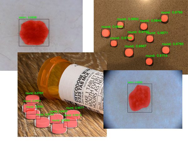
Figure 13: Inside my book, Deep Learning for Computer Vision with Python, you will learn how to annotate your own training data, train your custom Mask R-CNN, and apply it to your own images. I also provide two case studies on (1) skin lesion/cancer segmentation and (2) prescription pill segmentation, a first step in pill identification.

The Mask R-CNN model we used in this tutorial was pre-trained on the COCO dataset…

…but what if you wanted to train a Mask R-CNN on your own custom dataset?

Inside my book, Deep Learning for Computer Vision with Python, I:

1. Teach you how to train a Mask R-CNN to automatically detect and segment cancerous skinlesions — a first step in building an automatic cancer risk factor classification system.

2. Provide you with my favorite image annotation tools, enabling you to create masks for your input images.

3. Show you how to train a Mask R-CNN on your custom dataset.

4. Provide you with my best practices, tips, and suggestions when training your own Mask R-CNN.

All of the Mask R-CNN chapters included a detailed explanation of both the algorithm and code, ensuring you will be able to successfully train your own Mask R-CNNs.

To learn more about my book (and grab your free set of sample chapters and table of contents), just click here.

Summary

In this tutorial, you learned how to apply the Mask R-CNN architecture with OpenCV and Python to segment objects from images and video streams.

Object detectors such as YOLO, SSDs, and Faster R-CNNs are only capable of producing bounding box coordinates of an object in an image — they tell us nothing about the actual shape of the object itself.

Using Mask R-CNN we can generate pixel-wise masks for each object in an image, thereby allowing us to segment the foreground object from the background.

Furthermore, Mask R-CNNs enable us to segment complex objects and shapes from images which traditional computer vision algorithms would not enable us to do.

I hope you enjoyed today’s tutorial on OpenCV and Mask R-CNN!

To download the source code to this post, and be notified when future tutorials are published here on PyImageSearch, just enter your email address in the form below!

Downloads: