Classify your own images using Amazon SageMaker

Image classification and object detection in images are hot topics these days, thanks to a combination of improvements in algorithms, datasets, frameworks, and hardware. These improvements democratized the technology and gave us the ingredients for creating our own solution for image classification.

Object detection in images is one of the most important features of applications that do these activities, as shown in the image following:

• People pathing and object tracking

• Alerts for product repositioning in physical shops

• Visual search (searching using an image as input)

The state-of-the-art technologies for image classification and object detection are based on deep learning (DL). DL is a subarea of machine learning (ML) that is focused on algorithms for handling neural networks (NN) with many layers, or deep neural networks. ML, in turn, is a subarea of artificial intelligence (AI), a computer-science discipline.

Although anyone can access these technologies, it’s still hard to put the pieces together in an end-to-end solution that supports a real business process. Amazon Rekognition might be your first choice, given it is a ready to use service that offers a simple API that provides highly accurate facial analysis and facial recognition on your images and videos. Also, you can detect, analyze, and compare faces for a wide variety of user verification, people counting, and public safety use cases and more. Take a look on the Amazon Rekognition documentation and see how easy is to add all these features to you application with simple API calls.

However, if your business challenge requires a custom Image Classification, you’ll need a platform that supports the whole pipeline for creating your Machine Learning model. That’s what Amazon SageMaker was made for. Amazon SageMaker is a fully managed service that supports all of the steps of a ML model’s development: data exploration and building, training, and deploying ML models. With Amazon SageMaker, you can pick and use any of the built-in algorithms, reducing the time to market and the development cost. For more information, see Using Built-in Algorithms with Amazon SageMaker.

Creating a custom image classifier

Your goal in this blog post is to create an image classifier for identifying clothing pieces and accessories. You have several images of these items, and we want a model that can look at them and say (predict) what object each image contains. Amazon SageMaker already has a built-in image classification algorithm. With it, you just need to prepare your dataset (the image collection and the respective labels for each object) and start training your model.

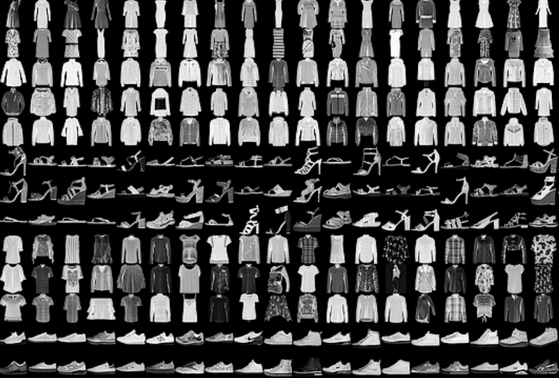
You’ll use a public dataset called Fashion-MNIST, a new image dataset for benchmarking ML algorithms. The dataset consists of a training set of 60,000 examples and a test set of 10,000 examples. Each example is a 28×28 grayscale image associated with a label or class. The dataset has 10 classes: T-shirt or top, trouser, pullover, dress, coat, sandal, shirt, sneaker, bag, and ankle boot. The following image shows a sample of the dataset.

You have the dataset and Amazon SageMaker for helping you train the fashion predictive model. But what computational resources do you need, and how long it will take to deploy the model in production?

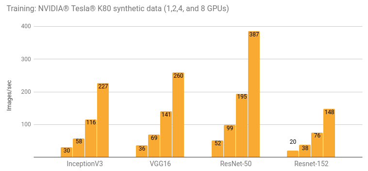
An instance like a p2.xlarge comes with NVIDIA Tesla K80 GPU, which has 12 GB of VRAM. GPUs are great for DL, whose training algorithms execute matrix operations like sums and multiplications. A GPU can execute these operations much faster than a CPU since GPUs have multiple cores specialized for parallel tasks. Tesla K80 training a Resnet152 (we’ll talk about that soon) can achieve about 20 images/second, as shown in the following performance graph.

Let’s suppose that you’re training your model with a dataset of 1M images and that you’ll need 100 epochs (or a single pass on the dataset by the training algorithm) to reach your target level of accuracy of 91%. With this setup, it would take about 14 hours per epoch or 58 days in total to complete the training.

Can you do better? Sure! How?

• Use a better GPU like NVIDIA Tesla V100 by changing the instance type from P2 to P3. Tesla V100 is 14 times faster than a K80. This upgrade can reduce the training time significantly.

• Use a P2 or P3 instance with more than one GPU. For example, a 16xlarge instance has eight V100 GPUs. You could divide your training workload by eight, proportionally reducing the time to market.

• Launch more than one training instance. Suppose that you have a huge dataset for training your model, and an instance with 8 GPUs is still taking more time than you can afford. You can tell Amazon SageMaker to execute a training job in two or more instances by setting the train_instance_count parameter of the tensorflow.TensorFlow class. Not only can you can parallelize your job inside an instance while distributing the load through several GPUs, but you can count on a farm of GPUs spread across multiple instances. For more information, see Step 2: Train a Model on Amazon SageMaker Using TensorFlow Custom Code.

• Apply a technique called transfer learning. Transfer learning uses a model that has already consumed several hours of training. You can customize it and retrain it to adapt it to your needs.

As you can see, you can configure Amazon SageMaker to provide an environment flexible enough to support your day-to-day ML pipeline scenario.

Understanding transfer learning

Before we move on, let’s look at Resnet, a NN topology that can achieve a high accuracy in image classification. It won the 2015 ImageNet Large Scale Visual Recognition Challenge for best object classifier, and it’s one of the most commonly used NNs for computer vision problems.

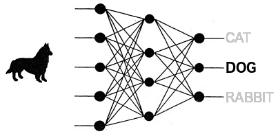
Topologies like Resnet are called a convolutional neural network (CNN) because the network’s input layers execute convolution operations on the input image. A convolution is a mathematical function that emulates the visual cortex of an animal. A CNN has several convolution layers that learn image filters. These filters extract features from the input images such as edges, parts, and bodies. These features are then routed through the hidden or inner layers to the output layer. In the context of image classification, the output layer has one output per category.

Consider a trained neural network capable of classifying a dog, as shown in the following image. The convolution layers extract some features from the dog image, and the rest of the layers route these features to the correct output of the last layer with a high confidence.

Transfer learning is a technique used for reducing the time required for training a new model. Instead of training your model from scratch, you can use a modified pre-trained model and continue training it with your dataset. That’s why it’s called transfer learning: the knowledge learned by one NN is transferring to another NN.

It means, for instance, that if you want a model that can classify cars brand/model/year and you already have a pre-trained model, it makes sense to change it a little bit and retrain it with your own dataset in order to create a new model that will solve this new problem.

The Amazon SageMaker built-in algorithm for image classification is already prepared for transfer learning. You just need to set a given parameter to true, and your model will use this technique.

Creating an end-to-end solution for image classification

You have an idea of which business problems you can solve with what you’ve seen so far, but how do you do it?

You can download the Jupyter notebook used in this hands on to see all the details of this experiment. Here we’ll see only the most relevant parts of this ML development pipeline for your fashion image classifier. The first step is preparing the dataset.

Preparing the dataset

The Amazon SageMaker built-in Image Classification algorithm requires that the dataset be formatted in RecordIO. RecordIO is an efficient file format that feeds images to the NN as a stream. Since Fashion MNIST comes formatted in IDX, you need to extract the raw images to the file system. Then you convert the raw images to RecordIO, and finally you upload them to Amazon Simple Storage Service (Amazon S3).

To prepare the dataset:

1. Download the dataset.

2. Unpack the images from IDX to raw JPEG grayscale images of 28×28 pixels.

3. Organize the images into 10 distinct directories, one per category.

4. Create two .lst files using a RecordIO tool (im2rec). One file is for the training portion of the dataset (70%). The other is for testing (30%).

5. Generate both .rec files from the .lst

6. Copy both .rec files to an Amazon S3 bucket.

For converting the dataset from IDX to raw JPEG files, you need to save the IDX files to a directory called samples and use a Python package called python-mnist.

pip install python-mnist

1 2 3 4 5 6 7 8 9 10 11 12 13 14

from mnist import MNIST from PIL import Image import numpy as np mndata = MNIST('samples') counter = 0 images, labels = mndata.load_training() for i, img in enumerate(images): img = np.reshape(img, (28, 28)) img = Image.fromarray(np.uint8(np.array(img))) img = img.convert("RGB") img.save('fashion_mnist/%s/img_%d.jpg' % (categories[labels[i]], counter )) counter += 1

read all the images from the directory fashion_mnist/ and create the .lst files

python $IM2REC –list=1 –recursive=1 –shuffle=1 –test-ratio=0.3 –train-ratio=0.7 fashion_mnist fashion_mnist/

read the .lst files and create the .rec files

python $IM2REC –num-thread=4 –pass-through=1 fashion_mnist_train.lst fashion_mnist python $IM2REC –num-thread=4 –pass-through=1 fashion_mnist_test.lst fashion_mnist

1 2 3 4 5 6 7 8 9 10 11 12 13 14 15 16 17 18 19 20 21 22 23 24 25 26 27 28 29 30 31 32 33 34 35 36 37 38 39 40 41 42 43 44 45 46 47 48 49 50 51 52 53 54 55 56 57 58 59 60 61 62 63 64 65 66 67 68 69 70 71 72 73 74 75 76

Then upload the .rec files to an Amazon S3 bucket. ### Set up the environment If you’re not familiar with Amazon SageMaker, read this blog post from Randall Hunt, an evangelist at AWS. It will give you a complete idea of how to set up a Jupyter notebook instance, which is our “cockpit” for creating our ML model. Make sure that the Role you attached to your Jupyter Notebook Instance has the privileges for accessing S3. That instance will read and write to chosen S3 bucket. Now it’s time to select the *hyperparameters* of your training environment. These parameters will determine how your model will be trained and, consequently, how your trained model will behave. - **num_layers:** the number of hidden/inner layers of your network. For small images chose a lower number, like [20, 32, 44, 56, 11]. - **image_shape:**number of channels per width and height pixels of the images. That is, 3,28,28 where 3 is the number of color channels (RGB) and 28,28 are the width and height pixels of the images. - **num_classes:** number of classes that the model can classify - **mini_batch_size:** the number of images each batch will contain. Depending on how much VRAM your GPU has you can increase or decrease this size. A large size can cause an out-of-memory exception and the training will fail. - **epochs:** how many times the training algorithm will pass through your whole dataset. Depending on the algorithm you chose, each epoch will get only a random sample of your dataset for each epoch. - **learning_rate:** how fast the training algorithm will try to optimize your model. Lower learning rates can achieve best accuracy will take more time to train your model. Higher learning rates can fail to improve your model accuracy. You need to find a good balance for this attribute. - **use_pretrained_model:** if set to 1 it will enable Transfer Learning. Amazon SageMaker will get a pretrained Resnet with Imagenet 11K categories and customize it to your scenario. After setting all these hyperparameters, you can select your instance, preferably a P2 or P3 instance with powerful GPUs, and start training your model. ### Training the model Amazon SageMaker is a platform based on Docker containers. Every built-in algorithm is a Docker image prepared with all of the libraries, frameworks, and binaries along with the algorithm itself. It turns the platform as flexible as possible. If you want to design your own ML algorithm, using your preferable technology just create a Docker image with your algorithm and call it from Amazon SageMaker. In this case, we will use an image that already contains the algorithm we need. This image will be used for creating a job that will train our model and then to publish the trained model in production as an endpoint. Depending on the region your Amazon SageMaker environment is running in, you’ll need to select a different registry: - **us-west-2:**dkr.ecr.us-west-2.amazonaws.com/image-classification:latest - **us-east-1:**dkr.ecr.us-east-1.amazonaws.com/image-classification:latest - **us-east-2:**dkr.ecr.us-east-2.amazonaws.com/image-classification:latest - **eu-west-1:**dkr.ecr.eu-west-1.amazonaws.com/image-classification:latest Next, you have to create a job description. The job description is a structure with all the parameters and hyperparameters you have set that will be sent to Amazon SageMaker so that SageMaker can then start a job for you. The result of this process is the trained model that will be saved to the S3 bucket you chose. You can monitor each step of the training process through CloudWatch Logs and Metrics, as shown in the following image. Just click in the running job in the Amazon SageMaker console and go to the Monitor session. If you want to see how much GPU memory is being utilized or what is the GPU or CPU utilization, just go to Amazon CloudWatch metrics.  Notice that the GPUMemoryUtilization is around 77%. A good GPU memory utilization is between 85% and 93%, so you can increase the batch size to speed up the training session. Amazon CloudWatch Logs will show you all the training algorithm output. You can see things like if your model is converging and how many batches/epochs were already processed.  In the preceding image, you can see the information “Validation-accuracy”. That is one of the most important pieces of information about the training. If the Train accuracy is too different from the Validation-accuracy, probably the model is overfitting, what is not good thing. A high “Validation-accuracy” indicates that the model is converging to a good format and can generalize well for new images that aren’t part of the training dataset. ### Testing and deploying the model Just to give you an idea, it took around 5 hours to train an Image Classifier with FashionMNIST in one p2 instance with just one GPU k80 with 40 epochs. In this particular case, the model reached an accuracy of 91, 10%, as you can see in CloudWatch Logs. However, it is important to mention that the training algorithm randomly selects portions of your dataset for each batch, instead of using the whole dataset per epoch. It improves the final performance but introduces a small variation in the training results from one job to another. It means that if I run several times the same training process it can reach that level of accuracy with less or more epochs. Depending on the business case, you may not need so accurate a model. Let’s say that 80% is good enough for your particular case. So, you can spend less time training and, consequently, there will be a cost reduction. On the other hand, if you need a high accurate model, you may need a larger dataset, for instance, and more epochs for converging your model, what would increase the training cost. As you can see, there is a trade off in this process. So, it is time to deploy that model in production. As you can see in the Jupyter notebook you’ll do that in 3 steps. 1. Convert the job output in a model that will be available in the Amazon SageMaker model catalog. 1. Create an endpoint configuration. In this step, you decide which instance will support your predictions. It is possible to train your model in a machine with GPU and then deploy it on a CPU only machine. That’s what we’ll do in our hands on. Deploying your model to a CPU only instance can reduce your costs. 1. Deploy your model, using the endpoint configuration defined previously. Amazon SageMaker will create an instance for you and deploy a container with the algorithm you’ve selected. Inside that container, your trained model will be hosted. After that, you will be able to send requests to that endpoint by using an API. Here’s an example of an API call for your deployed model:

import json import numpy as np import boto3 runtime = boto3.Session().client(service_name=’sagemaker-runtime’)

set the object categories array

object_categories = [‘AnkleBoot’,’Bag’,’Coat’,’Dress’,’Pullover’,’Sandal’,’Shirt’,’Sneaker’,’TShirtTop’,’Trouser’]

Load the image bytes

img = open(‘test_data/item1_thumb.jpg’, ‘rb’).read()

Call your model for predicting which object appears in this image.

response = runtime.invoke_endpoint( EndpointName=endpoint_name, ContentType=’application/x-image’, Body=bytearray(img) )

read the prediction result and parse the json

result = response[‘Body’].read() result = json.loads(result)

which category has the highest confidence?

pred_label_id = np.argmax(result)

print( “%s (%f)” % (object_categories[pred_label_id], result[pred_label_id] ) )

1 2 3 4 5 6

Running that code for a few sample images gives results like the following: 

Shirt (0.794700) TShirtTop (0.999502) AnkleBoot (0.999889) Sneaker (0.999952) Bag (0.795328)

1 2 3 4 5 6 7 8 9 10 11 12 13 14

Fashion-MNIST is composed by 28×28 grayscale images with black background. In a real business case scenario, you may need a dataset with larger and colored images to get a trained model that will be capable of classifying real clothes. The images above are not from the Fashion-MNIST. That’s why they were preprocessed to be as similar as possible to the images of the original dataset due to the original dataset restriction. An endpoint or a deployed model is also monitored by CloudWatch by default. You can click on the desired endpoint in the Amazon SageMaker console to see: - Runtime logs (CloudWatch Logs) - Invocation metrics (number of invocations, model latency, 4XX and 5XX errors, and so on) - Instance metrics (CPU/memory utilization and GPU/GPU memory utilization) The endpoint is protected by default. Nobody can call it until the user receives the correct privilege in the format of an AWS Identity and Access Management (IAM) policy. To allow a user to invoke your endpoint, you have to configure a policy like this:

{ “Version”: “2012-10-17”, “Statement”: [ { “Sid”: “VisualEditor0”, “Effect”: “Allow”, “Action”: “sagemaker:InvokeEndpoint”, “Resource”: “arn:aws:sagemaker:*:XXXXXXXXXXXX:endpoint/your-endpoint-name-here” } ] } ```

Another way to expose your endpoint to your application users is to encapsulate it in an API using API Gateway. You can delegate to API Gateway all of the security controls that you already defined to your applications and manage your environment the same way.

Conclusion

Amazon SageMaker helps you create a powerful solution for your image-classification needs. You can focus on the creation process and the business problem itself while Amazon SageMaker gives you a flexible and elastic infrastructure for supporting your ML pipeline.

Get a Jupyter notebook and start improving your application and your final users’ experience with a new image classifier.

 

---

About the Author

Samir Araújo is an AI Solutions Architect at AWS. He helps customers creating AI solutions for solving their business challenges, using the AWS platform. He has been working on several AI projects related to Computer Vision, Natural Language Processing, Inference, etc. He likes playing with hardware/programming projects in his free time and he has a particular interest for robotics.